It’s long been known that applying linear regression to equations transformed from nonlinear forms is generally not advisable. However, I had never actually examined how much the resulting values might differ in practice—so I decided to test it myself.
There are several methods that transform nonlinear equations into linear ones to estimate parameters. These include:
- Scatchard plot (used in ligand binding assays)
- Lineweaver–Burk plot (used in enzyme kinetics)
- Eadie-Hofstee plot
- Hanes–Woolf plot
Nowadays, these methods have been replaced by nonlinear regression, which is both far more accurate and easily accessible, so they should not be used except for data visualization purpose.
Avoid Scatchard, Lineweaver-Burke and similar transforms
Before nonlinear regression was readily available, the best way to analyze nonlinear data was to transform the data to create a linear graph, and then analyze the transformed data with linear regression. Examples include Lineweaver-Burke plots of enzyme kinetic data, Scatchard plots of binding data, and logarithmic plots of kinetic data. These methods are outdated, and should not be used to analyze data.
The problem with these methods is that the transformation distorts the experimental error. Linear regression assumes that the scatter of points around the line follows a Gaussian distribution and that the standard deviation is the same at every value of X. These assumptions are rarely true after transforming data. Furthermore, some transformations alter the relationship between X and Y. For example, in a Scatchard plot the value of X (bound) is used to calculate Y (bound/free), and this violates the assumption of linear regression that all uncertainty is in Y while X is known precisely. It doesn’t make sense to minimize the sum of squares of the vertical distances of points from the line, if the same experimental error appears in both X and Y directions.
Contents
Scatchard Equation and Plot
Derivation
Let’s assume an equilibrium between a receptor and a ligand as follows: $$ [R] + [L] \rightleftharpoons [RL] $$ The dissociation constant \(K_{\rm d}\) is defined as: $$K_{\mathrm d} = \frac{[R][L]}{[RL]} $$ Also, $$[R_{\mathrm T}] = [R] + [RL]$$ So, $$[RL] = \frac{[R_{\mathrm T}][L]}{K_{\mathrm d} + [L]} $$ This equation is a nonlinear expression equivalent to the Michaelis–Menten equation in enzyme kinetics. On the other hand, if we rearrange the same equation, we get: $$ \frac{K_{\mathrm d}[RL]}{[L]} = -[RL] + [R_{\mathrm T}] $$ Dividing both sides by \(K_{\rm d}\): $$\frac{[RL]}{[L]} = -\frac{1}{K_{\mathrm d}}[RL] + \frac{[R_{\mathrm T}]}{K_{\mathrm d}} $$ This is the Scatchard equation, which corresponds to the Eadie–Hofstee plot, a linear representation of the Michaelis–Menten equation.< From this equation, if you plot \([RL]\) on the x-axis and \([RL]/[L]\) on the y-axis, and perform linear regression, you will get a straight line where:
- The slope is \(-1/K_{\rm d}\)
- The x-intercept is \([R_{\rm T}]\)
Problems
The main problems with the Scatchard plot include:
- The x-axis (\([RL]\)) and y-axis (\([RL]/[L\)]) are not independent variables, since both contain \([RL]\).
- Least squares regression is fundamentally not applicable here, because it assumes:
- The x-axis is the explanatory variable (with no experimental error)
- The y-axis is the dependent variable (which contains experimental error)
- You cannot apply the correlation coefficient as a goodness-of-fit indicator.
- The method is indirect and extrapolative, rather than directly estimating parameters.
Practice Problem
I tried solving a practice problem from the lecture material archived at the following URL:
Mg2+ and ADP form a 1:1 complex. In the binding experiment, the total concentration of ADP is kept constant at 80 µM. From the data in the following table, determine the dissociation constant \(K_{\rm d}\).
| Total Mg2+ (µM) | Mg2+ bound to ADP (µM) |
| 20 | 11.6 |
| 50 | 26.0 |
| 100 | 42.7 |
| 150 | 52.8 |
| 200 | 59.0 |
| 400 | 69.5 |
First, from the equation \([RL] = \frac{[R_{\rm T}][L]}{(K_{\rm d} + [L]}\), we know that when \([L] = K_{\rm d}\), \([RL] = \frac{[R_{\rm T}]}{2} = 40\ \mbox{µM}\). So we can estimate that the \(K_{\rm d}\) is roughly around this value.
We analyze the data using R:。
#  R Software
> TotalMg = c(20, 50, 100, 150, 200, 400) # Total Mg2+
> B = c(11.6, 26.0, 42.7, 52.8, 59.0, 69.5) # Bound Mg<sup>2+</sup>, i.e., [RL]
> F = TotalMg - B # Free Mg²⁺, i.e., [L]
# Nonlinear regression
> result_nonlinear = nls(B ~ Rt*F/(Kd + F), start=c(Rt=10, Kd=10))
> summary(result_nonlinear)
Output:
Formula: B ~ Rt * F/(Kd + F)

Parameters:
   Estimate Std. Error t value Pr(>|t|)
Rt 79.92642    0.08296   963.5 6.96e-12 ***
Kd 49.86861    0.15975   312.2 6.32e-10 ***
---
Signif. codes:  0 ‘***’ 0.001 ‘**’ 0.01 ‘*’ 0.05 ‘.’ 0.1 ‘ ’ 1

Residual standard error: 0.05816 on 4 degrees of freedom

Number of iterations to convergence: 5
Achieved convergence tolerance: 1.579e-06

> confint(result_nonlinear)
Waiting for profiling to be done...
       2.5%    97.5%
Rt 79.69637 80.15752
Kd 49.42630 50.31459
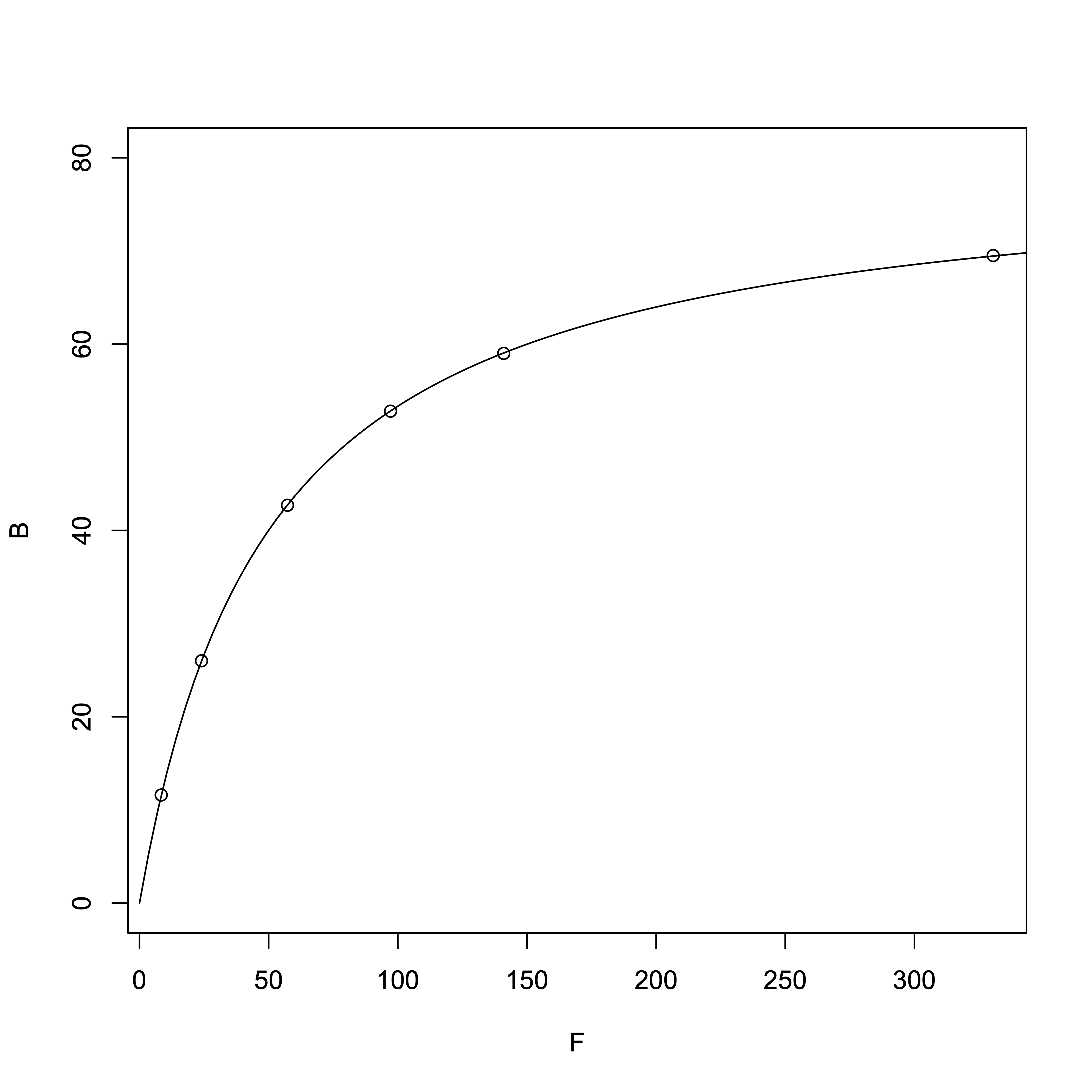
From the nonlinear regression, we obtained:
- Dissociation constant \(K_{\rm d}\) = 49.87 µM
- \([R_{\rm T}]\) = 79.93 µM
Now, using the Scatchard plot to determine \(K_{\rm d}\) and \([R_{\rm T}]\):
# R Software
> result_linear = lm(B/F ~ B)
> summary(result_linear)
Output:
Call:
lm(formula = B/F ~ B)
Residuals:
         1          2          3          4          5          6
 0.0038911 -0.0026571 -0.0032285 -0.0010654 -0.0005134  0.0035734
Coefficients:
              Estimate Std. Error t value Pr(>|t|)
(Intercept)  1.6115350  0.0033919   475.1 1.18e-10 ***
B           -0.0202132  0.0000709  -285.1 9.08e-10 ***
---
Signif. codes:  0 ‘***’ 0.001 ‘**’ 0.01 ‘*’ 0.05 ‘.’ 0.1 ‘ ’ 1
Residual standard error: 0.00342 on 4 degrees of freedom
Multiple R-squared:      1,	Adjusted R-squared:  0.9999
F-statistic: 8.128e+04 on 1 and 4 DF,  p-value: 9.081e-10
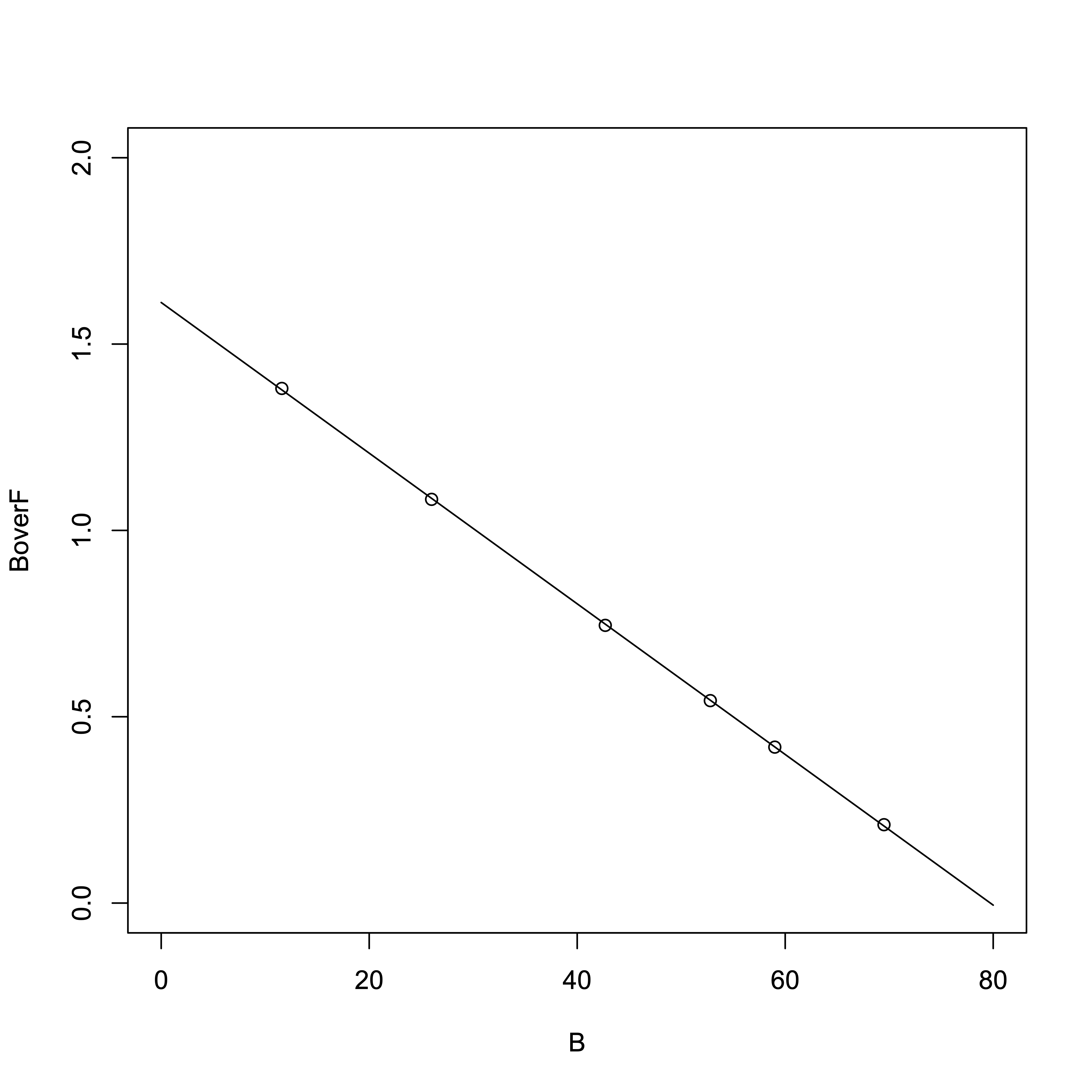
From the regression line:
- Slope = \(-1/K_{\rm d}\) = -0.0202132
- x-intercept (i.e., \([R_{\rm T}]\)) = –y-intercept / slope = 1.6115350 / 0.0202132
- \(K_{\rm d}\) = 49.47 µM
- \([R_{\rm T}]\) = 79.72 µM
This exercise used \(K_{\rm d}\) = 50 µM to generate the data points. However, rounding of the bound Mg2+ values introduces small errors, which result in slight differences in the \(K_{\rm d}\) and \([R_{\rm T}]\) values obtained via nonlinear regression and the Scatchard method. When you calculate using values rounded to the second decimal place, you get results very close to the theoretical ones:
- Nonlinear regression: \(K_{\rm d}\) = 49.99 µM
- Scatchard method: \(K_{\rm d}\) = 49.97 µM
Actual Data
In the previous practice problem using idealized values, there was almost no difference between the results obtained via nonlinear regression and the Scatchard plot. Now, I tried applying both methods to real experimental data to see how they compare.
> B = c(0.729,0.805,0.748,1.328,1.317,1.314,1.905,1.936,1.851,2.546,2.414,2.355) # Units: nM
> F = c(6.102,5.532,5.490,10.448,11.710,11.092,22.863,24.570,24.401,48.750,46.621,46.682) # Units: nM
> result = nls(B~Rt*F/(Kd+F),start=c(Rt=3,Kd=0.2))
> summary(result)
Output:
Formula: B ~ Rt * F/(Kd + F)

Parameters:
   Estimate Std. Error t value Pr(>|t|)
Rt   3.3825     0.1127   30.01 3.95e-11 ***
Kd  18.3799     1.4360   12.80 1.59e-07 ***
---
Signif. codes:  0 ‘***’ 0.001 ‘**’ 0.01 ‘*’ 0.05 ‘.’ 0.1 ‘ ’ 1

Residual standard error: 0.06848 on 10 degrees of freedom

Number of iterations to convergence: 6
Achieved convergence tolerance: 1.785e-07

> confint(result) # 95% confidence interval
Waiting for profiling to be done...
        2.5%     97.5%
Rt  3.148358  3.652665
Kd 15.470323 21.906326
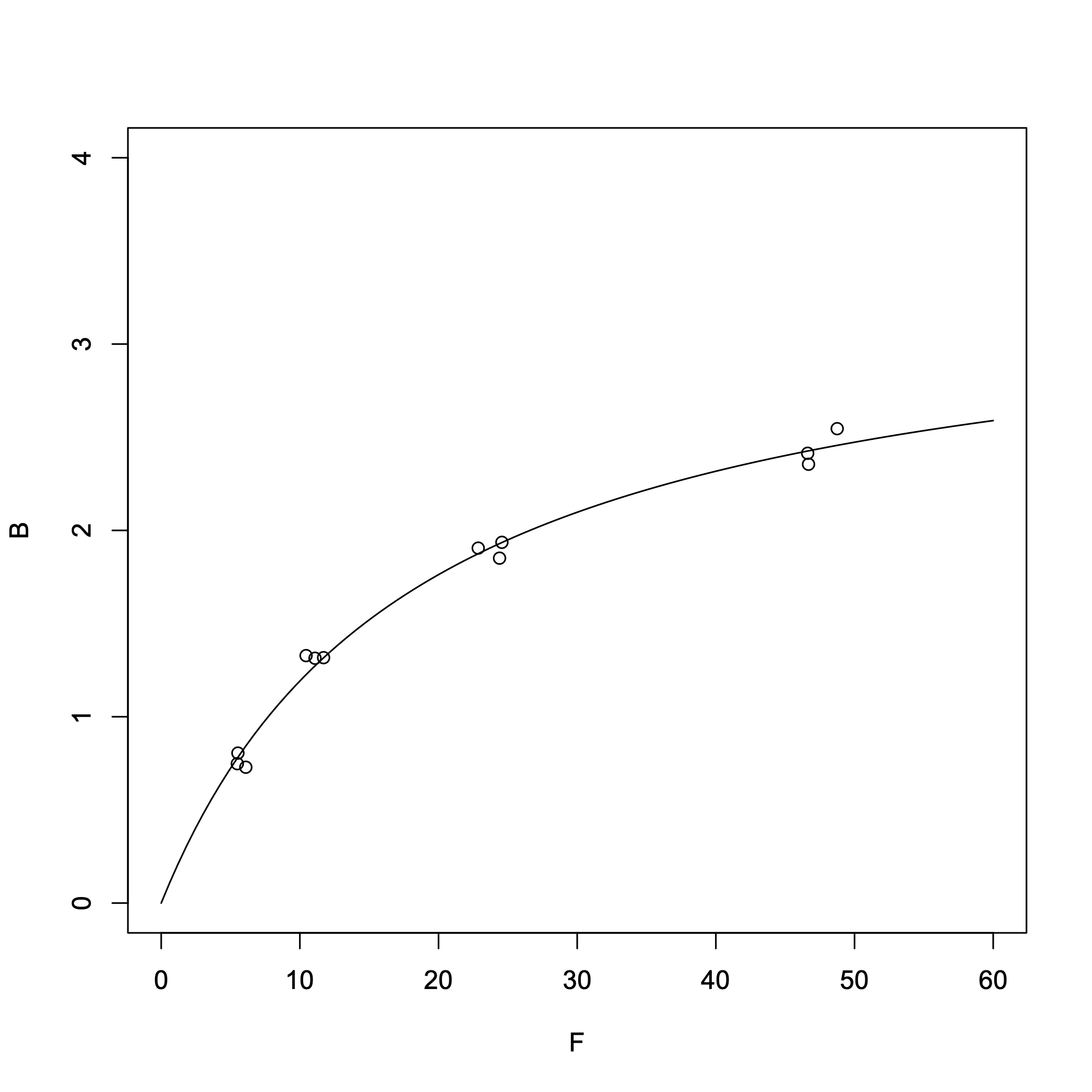
From the nonlinear regression, we obtained:
- Dissociation constant \(K_{\rm d}\) = 18.4 nM
- \([R_{\rm T}]\) = 3.38 nM
> result_lm = lm(B/F ~ B)
> summary(result_lm)
Output:
Call:
lm(formula = B/F ~ B)

Residuals:
       Min         1Q     Median         3Q        Max
-0.0207551 -0.0043123  0.0007946  0.0048720  0.0171733

Coefficients:
             Estimate Std. Error t value Pr(>|t|)
(Intercept)  0.177090   0.008028   22.06 8.21e-10 ***
B           -0.050571   0.004659  -10.85 7.46e-07 ***
---
Signif. codes:  0 ‘***’ 0.001 ‘**’ 0.01 ‘*’ 0.05 ‘.’ 0.1 ‘ ’ 1

Residual standard error: 0.01015 on 10 degrees of freedom
Multiple R-squared:  0.9218,	Adjusted R-squared:  0.9139
F-statistic: 117.8 on 1 and 10 DF,  p-value: 7.464e-07
> confint(result_lm)
                  2.5 %     97.5 %
(Intercept)  0.15920357  0.1949766
B           -0.06095189 -0.0401892
> -1/result_lm$coefficients[2]
       B
19.77436
> -result_lm$coefficients[1]/result_lm$coefficients[2]
(Intercept)
   3.501842
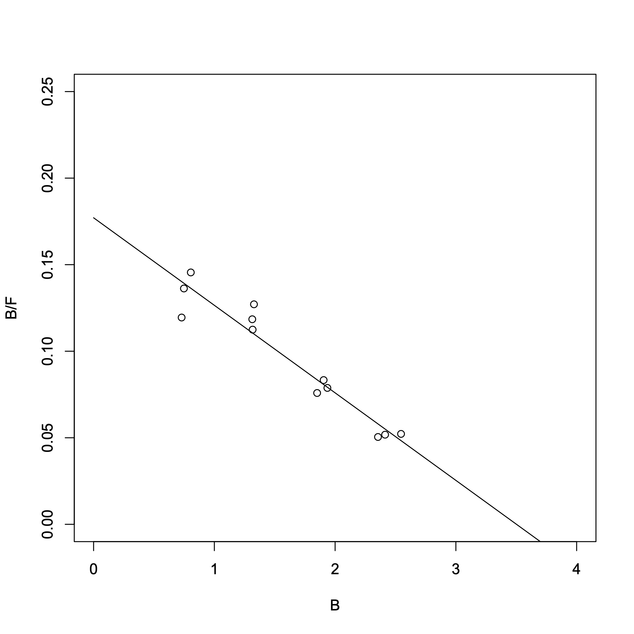
The two lowest-concentration B/F values overlap in range. (Because the inverse of F is used, the error becomes significantly amplified.) From the Scatchard plot, we obtained:
- Dissociation constant \(K_{\rm d}\) = 19.8 nM
- \([R_{\rm T}]\) = 3.50 nM
Comparing the 95% confidence intervals for \(K_{\rm d}\):
- Nonlinear regression: \(K_{\rm d}\) = 18.4 nM (95% CI: 15.5–21.9)
- Scatchard plot: \(K_{\rm d}\) = 19.8 nM (95% CI: 16.4–24.9)
References
- Braun, Derek C.; Garfield, Susan H.; Blumberg, Peter M. “Analysis by Fluorescence Resonance Energy Transfer of the Interaction between Ligands and Protein Kinase Cδ in the Intact Cell”. J. Biol. Chem. 2005, 280(9), 8164-8171. doi: 10.1074/jbc.M413896200
- Scatchard, George “The Attraction of Proteins for Small Molecules and Ions”. Annals of the New York Academy of Sciences 1949, 51(4), 660–672. doi: 10.1111/j.1749-6632.1949.tb27297.x.