In the world of drug discovery, where scientists are the detectives and diseases are the elusive criminals, radioligand binding assays (RLBAs) were once the Sherlock Holmes of the lab.
— Ancellin, Nicolas, “Radioligand Binding Assays: A Lost Art in Drug Discovery?”.
Memo.Translated on May 13, 2025.
Several methods exist for calculating the inhibition constant (\(K_{\mathrm i}\)). Besides the widely known Cheng–Prusoff equation, modified Cheng–Prusoff equation using [L]50 value instead of [L]T, and the exact Munson–Rodbard correction, which allows direct calculation using the total concentration of an unlabeled ligand—namely, the 50% inhibitory concentration \({\rm IC}_{50}\)—without requiring approximations. Additionally, the 50% inhibitory concentration of the free ligand, denoted \([I]_{50}\), can be estimated either via nonlinear regression or linear regression.
We investigates the deviation between the estimated \(K_{\rm i}\) values obtained by these methods and the true \(K_{\rm i}\) values using simulated data.
To simulate realistic assay conditions, typical experimental values were used for the binding between the protein kinase C δ-C1B domain (as receptor) and the radiolabeled ligand [³H]phorbol 12,13-dibutyrate ([³H]PDBu):
- Total receptor concentration: \([R]_{\rm T}\) = 3.45 nM
- Total radioligand concentration: \([L]_{\rm T}\) = 17 nM
- Radioligand dissociation constant: \(K_{\rm d}\) = 0.53 nM
For various true values of \(K_{\rm i}\), the ranges of total unlabeled ligand concentration \(\log_{10} [I]_{\rm T}\) used in the simulations were:
- \(K_{\rm i}\) = 0.05 nM: from −9.021 to −7.457
- \(K_{\rm i}\) = 0.1 nM: from −9.172 to −7.459
- \(K_{\rm i}\) = 0.5 nM: from −8.908 to −6.987
- \(K_{\rm i}\) = 1 nM: from −8.454 to −6.496
- \(K_{\rm i}\) = 10 nM: from −7.495 to −5.500
- \(K_{\rm i}\) = 100 nM: from −6.500 to −4.500
(Five data points spaced approximately 0.5 log units apart, centered around the expected 50% inhibition point.)
There was no significant difference between the results of nonlinear regression (fitting to a standard sigmoid function) and linear regression (after logit transformation) in estimating \({\rm IC}_{50}\):
| True Ki | [I]50 (nM) | True IC50 (nM) | IC50 ( from nonlinear regression) | IC50 (from linear regression) |
| 0.05 nM | 1.51 | 3.24 | 3.18 | 3.17 |
| 0.1 nM | 3.02 | 4.75 | 4.71 | 4.68 |
| 0.5 nM | 15.1 | 16.8 | 16.8 | 16.8 |
| 1 nM | 30.2 | 31.9 | 31.9 | 31.9 |
| 10 nM | 302 | 304 | 303 | 303 |
| 100 nM | 3019 | 3020 | 3015 | 3014 |
| True Ki | Ki (nM) calculated from True IC50 | |||
| Cheng–Prusoff | Cheng–Prusoffa | Munson–Rodbard (exact) correction | IC50 – [R]T/2 correctionb | |
| 0.05 nM | 0.0980 | 0.108 | 0.500 | 0.502 |
| 0.1 nM | 0.143 | 0.159 | 0.100 | 0.100 |
| 0.5 nM | 0.508 | 0.561 | 0.499 | 0.499 |
| 1 nM | 0.964 | 1.07 | 1.00 | 1.00 |
| 10 nM | 9.19 | 10.2 | 10.0 | 10.0 |
| 100 nM | 91.3 | 101 | 100 | 100 |
| a Using [L]50 instead of [L]T 。 b \(K_{\mathrm i} = (\mathrm{IC}_{50} – [R]_\mathrm{T}/2 )/(2 [L]_{50}/[L]_{0} – 1 + [L]_{50}/K_\mathrm{d}) \). | ||||
Conclusions
The original Cheng–Prusoff equation shows unexpectedly large deviations even when the \(K_{\mathrm i}\) value is high.
Modified Cheng–Prusoff equation using \([L]_{50}\) agrees with the true \(K_{\rm i}\) value to two significant digits when \(K_{\rm i}\) ≥ 10 nM.
Nowadays, when spreadsheet software is available, there is no reason not to use the exact Munson–Rodbard correction. At least in cases where \(K_{\mathrm i} < 10\) nM, where the difference between \([I]_{50}\) and \(\mathrm{IC}_{50}\) widens, it is necessary to use the Munson–Rodbard equation.
- In practice, the Ki value obtained using the approximation \([I]_{50} \simeq \mathrm{IC}_{50} – [R]_{\mathrm T}/2 \) is sufficiently accurate.
Contents
Binding Assay Calculations
The binding assay methodology is based on Sharkey & Blumberg (1985), with modifications. Non-specific binding at equilibrium is neglected. Key equations include:
- Specific binding: $$[RL]_0 =[\mbox{pellet(total)}] – k \times [\mbox{supernatant(total)}]\times \frac{437}{50} $$
- Partition Coefficient k: $$\mathbf{\mathit{k}} = \frac{[\mbox{pellet(nonspecific)}]}{[\mbox{supernatant(nonspecific)}] \times \frac{437}{50}}$$
- Total Ligand Concentration: $$\mathbf{[\mathit{L}]_{\mathrm T}} = [\mbox{pellet(total)}] + [\mbox{supernatant(total)}] \times \frac{437}{50}$$
- Corrected Total Ligand Concentration: $$\mathbf{[\mathit{L}]^{*}_{\mathrm T}} =\frac{[L]_{\mathrm T}}{1 + k}$$
- Free Ligand Concentration: $$\mathbf{[\mathit{L}]_0} = [\mbox{supernatant(total)}] = \frac{[L]_{\mathrm T} − [RL]_0}{1 + k}$$
- Ligand Concentration at 50% Binding: $$\mathbf{[\mathit{L}]_{50}} = \frac{[L]_{\mathrm{T}} − \frac{[RL]_0}{2}}{1 + k}$$
- Total Receptor Concentration: $$\mathbf{[\mathit{R}]_\mathrm{T}} = \frac{K_\mathrm{d} [RL]_0}{[L]_0 + [RL]_0}$$
- Conversion Factor N from DPM to nM:: $$N = \frac{1}{60} \times \frac{1}{3.7 \times 10^{10}} \times \frac{1}{\mbox{specific activity (Ci/mmol)}} \times \frac{1}{10^3} \times \frac{1}{250 \times 10^{-6}} \times 10^9$$
Non-Specific Binding Considerations
In membrane preparations, non-specific binding can occur due to low-affinity interactions with membrane proteins, phospholipid partitioning, or filter adsorption. These are typically unsaturable and modeled as the product of the non-specific binding coefficient \(k\) and the free radioligand concentration \([L]\) (Hulme and Trevethick, 2010).
In [3H]PDBu binding assays, polyethylene glycol (PEG) is added to precipitate proteins, with γ-globulin included as a co-precipitant, leading to non-specific adsorption (typically \(k = 3–5\%\)). Calculations show that at \(k = 0\), \([RL]_0 = 3.321\ \mbox{nM}\) and \([L]_0 = 13.7\ \mbox{nM}\); at \(k = 0.04\), \([RL]_0 = 3.316\ \mbox{nM}\) and \([L]_0 = 13.2\ \mbox{nM}\). High ligand concentrations minimize the impact on bound \([RL]\), allowing correction of free \([L]\) using \(k\).
For unlabeled ligands, if the partition coefficient is assumed equal to that of [3H]PDBu, adjusting the added concentration by dividing by \(1 + k\) provides a good estimate of \([I_\mathrm{T}]\). For example, with a true \(K_\mathrm{i} = 10\ \mbox{nM}\) and \(k = 0.04\), the apparent \(K_\mathrm{i}\) calculated using the Munson–Rodbard equation is \(10.47\ \mbox{nM}\) without correction and \(10.06\ \mbox{nM}\) with correction.
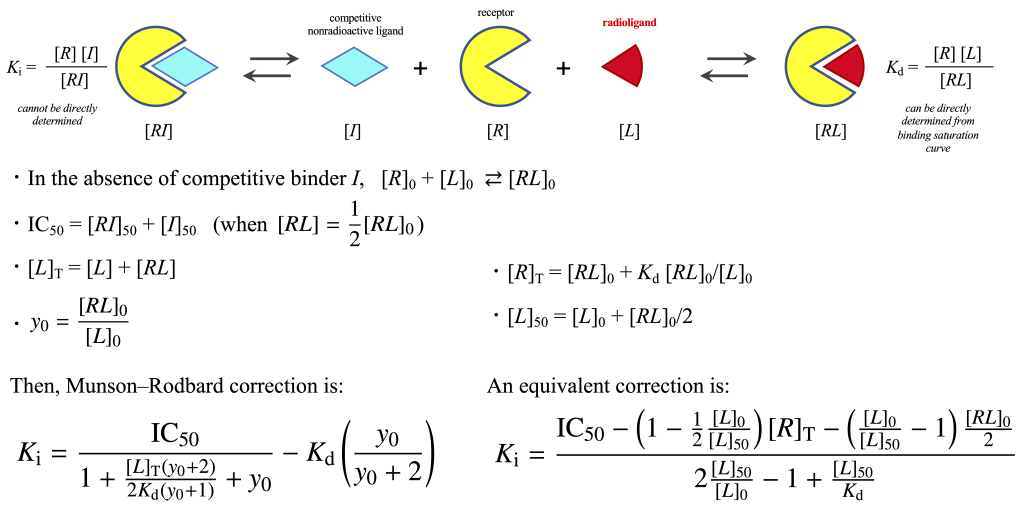
Cheng–Prusoff equation
Parameters Used
Total Binding Group:
$$[R]_0 + [L]_0 \rightleftharpoons [RL]_]$$ $$K_{\rm d} = \frac{[R]_0[L]_0}{[RL]_0}$$ $$[R]_{\rm T} = [R]_0 + [RL]_0$$ $$K_{\rm d} = \frac{([R]_{\rm T} – [RL]_0)[L]_0}{[RL]_0}$$ $$[RL]_0 = \frac{[R]_{\rm T}[L]_0}{K_{\rm d} + [L]_0}$$
Competitive Inhibition Group:
\([I]\): Concentration of free, non-labeled ligand
$$[RI] \rightleftharpoons [I] + [R] + [L] \rightleftharpoons [RL]$$ $$K_{\rm i} = \frac{[R][I]}{[RI]}$$ $$[R]_{\rm T} = [RI] + [R] + [RL]$$ $$[R]_{\rm T}= \frac{[R][I]}{K_{\rm i}} + [R] + [RL]$$ $$[R]_{\rm T}= \left(1+\frac{[I]}{K_{\rm i}}\right)[R] + [RL]$$ $$[R]_{\rm T} = \left(1+\frac{[I]}{K_{\rm i}}\right)\frac{K_{\rm d}[RL]}{[L]}+ [RL]$$ $$[RL] = \frac{[R]_{\rm T}[L]}{\left(1+\frac{[I]}{K_{\rm i}}\right)K_{\rm d} + [L]}$$
At 50% Inhibition of Binding
Let us consider the situation at 50% inhibition of binding: $$\frac{1}{2}[RL]_0 = [RL]_{50}$$ $$\frac{1}{2}\frac{[R]_{\rm T}[L]_0}{K_{\rm d} + [L]_0} = \frac{[R]_{\rm T}[L]_{50}}{\left(1+\frac{[I]_{50}}{K_{\rm i}}\right)K_{\rm d} + [L]_{50}}$$ Multiply both sides and rearrange: $$2\frac{K_{\rm d} }{[L]_0} + 2 = \left(1+\frac{[I]_{50}}{K_{\rm i}}\right)\frac{K_{\rm d} }{[L]_{50}}+ 1$$ $$2\frac{[L]_{50}}{[L]_0} + \frac{[L]_{50}}{K_{\rm d}} = 1+\frac{[I]_{50}}{K_{\rm i}}$$ Solving for \(K_{\rm i}\): $$K_{\rm i} = \frac{[I]_{50}}{2\frac{[L]_{50}}{[L]_0} – 1 + \frac{[L]_{50}}{K_{\rm d}}} \;\;\;\mbox{(Goldstein and Barrett, 1987)}$$ $$= \frac{[I]_{50}}{1 + \frac{[L]_{50}}{K_{\rm d}} + 2\frac{[L]_{50}-[L]_0}{[L]_0}}$$
Conversion to Cheng–Prusoff Equation
If the ligand concentration \([L]\) is sufficiently large compared to receptor concentration \([R]\), then \([L]_0 \simeq [L]_{50} \simeq [L]^{*}_{\rm T}\), so $$K_{\rm i} = \frac{[I]_{50}}{1 + \frac{[L]^{*}_{\rm T}}{K_{\rm d}}}\;\; .$$
If the inhibitor concentration \([I]\) is sufficiently large compared to the receptor concentration \([R]\), \([I]_{50}\) can be approximated as the total ligand concentration at 50% inhibition, i.e., \(\rm{IC}_{50}\):
$$K_{\rm i} = \frac{\textrm{IC}_{50}}{1+\frac{[L]^{*}_{\rm T}}{K_{\rm d}}} \;\;\;\mbox{(Cheng–Prusoff equation)}\;\; .$$
Drawing Binding Inhibition Curve
The value of \([RL]_0\) can be obtained by solving a quadratic equation
$$ [RL]_0 = \frac{1}{2}\left[([R]_{\rm T} + [L]_{\rm T} + K_{\rm d}) – \sqrt{([R]_{\rm T} + [L]_{\rm T} + K_{\rm d})^2 – 4[R]_{\rm T}[L]_{\rm T}}\right] \; .$$
When \([R]_\mathrm{T}=3.45\), \([L]_\mathrm{T}=17\), and \(K_\mathrm{d}=0.53\), \([RL]_0=3.321\).
Similarly, in the presence of an unlabeled ligand, \([RL]\) can be expressed as the following function of the free unlabeled ligand concentration \([I]\):
$$ [RL] = \frac{1}{2}\left\{\left[[R]_{\rm T} + [L]_{\rm T} + \left(1+\frac{[I]}{K_{\rm i}}\right)K_{\rm d}\right] – \sqrt{\left[[R]_{\rm T} + [L]_{\rm T} + \left(1+\frac{[I]}{K_{\rm i}}\right)K_{\rm d}\right]^2 – 4[R]_{\rm T}[L]_{\rm T}}\right\} $$
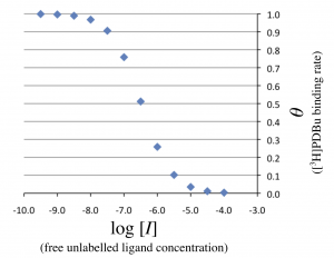
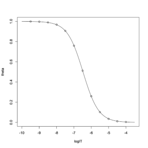
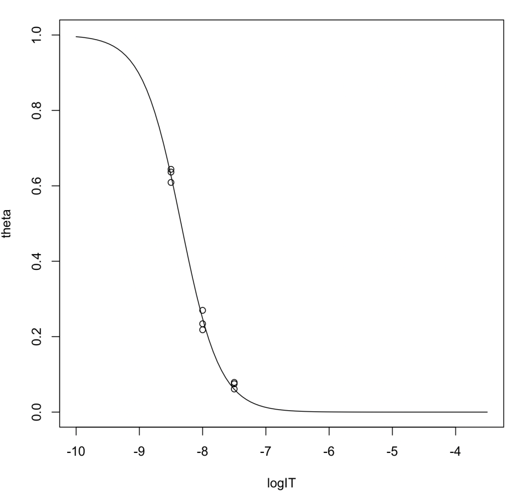
When the fractional radioligand binding
$$\theta = [RL]/[RL]_0$$
is plotted against the free unlabeled ligand concentration \(\log_{10}[I]\), the following graph can be obtained.
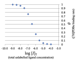
Then, the horizontal axis in Figure 1 is changed to \(\log_{10} [I]_{\rm T}\), the logarithmic total concentration of unlabeled ligand. Note that $$ [I]_{\mathrm T} = [I] + [RI] $$
and
$$ [RI] = [R]_{\mathrm{T}} – \frac{[L]_0}{[L]_{\mathrm T} – [RL]}\frac{[RL]}{[RL]_0}[R]_{\mathrm{T}} + \left( \frac{[L]_0}{[L]_{\mathrm T} – [RL]} – 1\right) [RL] \;\; .$$
data.csv
logIT,theta
-9.495,0.999
-8.995,0.997
-8.495,0.990
-7.995,0.968
-7.496,0.906
-6.996,0.759
-6.498,0.512
-5.999,0.259
-5.500,0.102
-5.000,0.035
-4.500,0.011
-4.000,0.004
Estimating \({\rm IC}_{50}\)by Regression
Nonlinear Regression
1) Fitting to the Complementary Error Function (erfc)
Fitting to the complementary error function (erfc)
$$\operatorname{erfc}(x)=\frac{2}{\sqrt{\pi}} \int_{x}^{\infty} e^{-t^2}dt$$
The probit function is the inverse function of the cumulative distribution function \(\Phi\) of the normal distribution. The complementary error function, erfc, and \(\Phi\) are related by the following expression:
$$\Phi(x)=\frac{1}{2}\operatorname{erfc} \left(-\frac{x}{\sqrt{2}}\right) \; .$$
> simulation <- read.csv("data.csv")
> erfc <- function(x) 2 * pnorm(x * sqrt(2), lower=FALSE)
> result2 = nls(theta~1/2*erfc((logIT - logIC50)/a), data = simulation, start = c(logIC50=-6.5, a=1))
> summary(result2)
Formula: $$\theta = \frac{1}{2}\cdot\operatorname{erfc}\left(\frac{\log_{10}[I]_{\rm T} - \log_{10}{\rm IC}_{50}}{a}\right)$$
(Note: The complementary error function is multiplied by 1/2 to constrain the range between 0 and 1)
Output:
Formula: theta ~ 1/2 * erfc((logIT - logIC50)/a)

Parameters:
         Estimate Std. Error t value Pr(>|t|)
logIC50 -6.476263   0.006851 -945.27  < 2e-16 ***
a        1.082295   0.013710   78.94  2.6e-15 ***
---
Signif. codes:  0 ‘***’ 0.001 ‘**’ 0.01 ‘*’ 0.05 ‘.’ 0.1 ‘ ’ 1

Residual standard error: 0.005889 on 10 degrees of freedom

Number of iterations to convergence: 5
Achieved convergence tolerance: 6.534e-07
Visualizing Fit:
> concpre = seq(-10,-3.5, length=100)
> plot(theta~logIT,data=simulation,xlim=c(-10,-3.5),ylim=c(0,1))
> lines(concpre, predict(result2, newdata=list(logIT=concpre)))
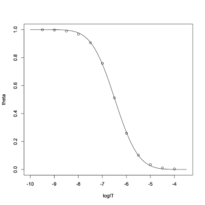
The fit is not very good.
2) Fitting to a decreasing logistic function \(1/(1 + \exp(ax))\):
The standard sigmoid function is
$$f(x)=\frac{1}{1+e^{-ax}}\; .$$
The decreasing logistic function is defined as 1 minus the standard sigmoid function:
$$f(x)=1-\frac{1}{1+e^{-ax}}=\frac{1}{1+e^{ax}}\; .$$
> result3 = nls(theta~1/(1+exp(a*log(10)*(logIT - logIC50))), data = simulation, start = c(logIC50=-6.5, a=1))
> summary(result3)
Formula: $$\theta = \frac{1}{1 + e^{a \log_{e} 10 (\log_{10}[I]_{\rm T} - \log_{10}{\rm IC}_{50})}}$$
Output:
Formula: theta ~ 1/(1 + exp(a * log(10) * (logIT - logIC50)))

Parameters:
         Estimate Std. Error t value Pr(>|t|)
logIC50 -6.476238   0.001243 -5209.7   <2e-16 ***
a        0.964276   0.002346   411.1   <2e-16 ***
---
Signif. codes:  0 ‘***’ 0.001 ‘**’ 0.01 ‘*’ 0.05 ‘.’ 0.1 ‘ ’ 1

Residual standard error: 0.001071 on 10 degrees of freedom

Number of iterations to convergence: 4
Achieved convergence tolerance: 8.128e-08
The simulation data appear to fit the decreasing logistic function perfectly. The estimated values were \(\log_{10}\mathrm{IC}_{50}= -6.476238\) and \(a=0.964276\). This curve is referred to as an inhibition curve in the fields of biology and pharmacology. The parameter \(a\) corresponds to the ligand Hill coefficient \(n_{H}\), which describes the slope of the sigmoidal curve. The transformation is shown below.
First, as shown two sections below, \(\theta\) can be written as
$$\theta = \frac{\frac{[L]}{[L]_0} (K_{\rm d} + [L]_0)}{\frac{K_{\rm d}}{K_{\rm i}}[I] + K_{\rm d} + [L]} \; .$$
If \([L] \simeq [L]_0\) and \([I] \simeq [I]_{\mathrm T}\),
$$\theta = \frac{1}{1 + \frac{1}{K_{\rm d} + [L]_0}\frac{K_{\rm d}}{K_{\rm i}} [I]_{\mathrm T}} \; .$$
This can be rewritten as
$$\theta = \frac{1}{1 + \exp\left\{\log_{e} 10 \left[\log_{10} [I]_{\mathrm T} - \log_{10} K_{\mathrm i}\left( 1+ \frac{[L]_0}{K_\mathrm{d}} \right) \right]\right\}} \; .$$
From the Cheng–Prusoff equation,
$$ K_{\mathrm i}\left( 1+ \frac{[L]_0}{K_\mathrm{d}} \right) \simeq \mathrm{IC}_{50}\; ,$$
and therefore \(\theta\) can be approximated as
$$\theta = \frac{1}{1 + \exp\left[\log_{e} 10 \left(\log_{10} [I]_{\mathrm T} - \log_{10} \mathrm{IC}_{50} \right)\right]} \; .$$
In practice, nearly identical IC50 values are obtained even when the complementary error function is used; however, this formulation provides a superior model.
Linear Regression
Next, to visually evaluate the goodness of fit of the fitted curve, a transformation to a linear graph (e.g., for use in Microsoft Excel) is shown.
From the following expression: $$\frac{\theta}{1-\theta} = \frac{\frac{[L]}{[L]_0}(K_{\rm d} + [L]_0)}{\frac{K_{\rm d}}{K_{\rm i}}[I] + K_{\rm d} + [L] - \frac{[L]}{[L]_0}(K_{\rm d} + [L]_0)} = \frac{\frac{[L]}{[L]_0} K_{\rm d} + [L]}{\frac{K_{\rm d}}{K_{\rm i}}[I] + \left(1 - \frac{[L]}{[L]_0}\right) K_{\rm d}} $$
Assuming \([L]_0 \simeq [L]\), it simplifies to: $$\frac{\theta}{1-\theta} = \frac{K_{\rm d} + [L]}{\frac{K_{\rm d}}{K_{\rm i}}[I]}$$
Taking the logarithm (base 10): $$\log \left(\frac{\theta}{1-\theta}\right) = -\log [I] -\log K_{\rm d} + \log K_{\rm i} + \log (K_{\rm d} + [L])$$ This results in a linear relationship with a slope of \(-1\) when plotted against \(\log[I]\) (free ligand concentration) (logit function) (Figure 3).
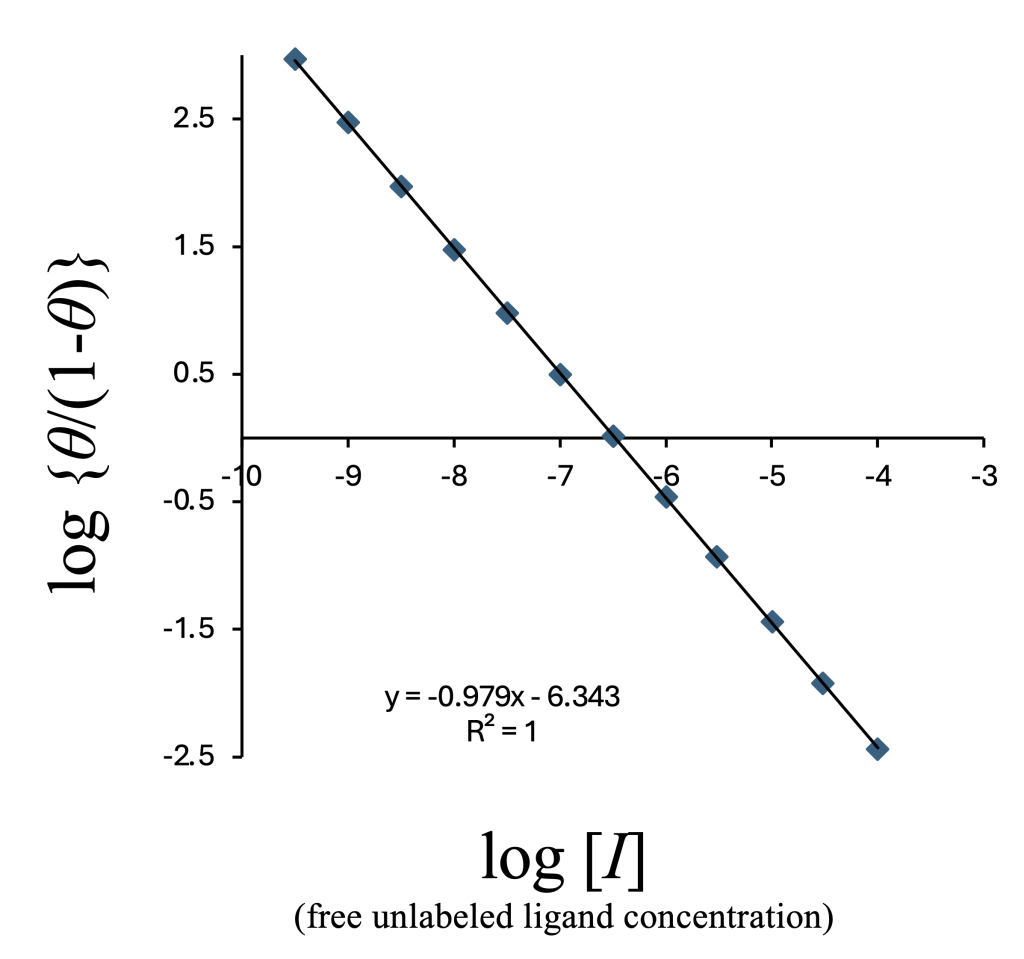
Although the horizontal axis in the figure above is \(\log[I]\) (free unlabeled ligand), this value is not experimentally accessible. Instead, we use the added total ligand concentration \(\log[I]_{\rm T}\), and obtain:
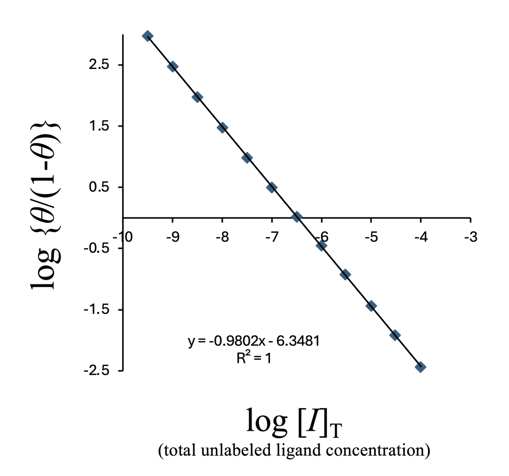
- \(\log{\rm IC}_{50} = -6.4765\) from the linear plot
- \(\log{\rm IC}_{50} = -6.4762\) from nonlinear regression using the standard sigmoid function.
These values match up to four significant digits. In nM units:
- 333.8 nM (from linear regression),
- 334.0 nM (from nonlinear regression).
Simple Conversion from Binding Ratio to \(K_{\rm i}\)
For weak ligands that do not inhibit binding by more than 50%, \(K_{\rm i}\) can be calculated from a single data point using the following rearranged form:
$$\frac{\theta}{1-\theta} = \frac{K_{\rm d} + [L]}{\frac{K_{\rm d}}{K_{\rm i}}[I]} \rightarrow K_{\rm i} = \left(\frac{\theta}{1-\theta}\right) \frac{K_{\rm d}[I]}{K_{\rm d} + [L]}\;\; .$$
If the unlabeled ligand concentration \([I]\) is sufficiently large compared to the receptor concentration \([R]\) (which is the case for weak ligands), \([I]\) can be approximated by the total ligand concentration \([I]_{\rm T}\).
$$K_{\rm i} = \left(\frac{\theta}{1-\theta}\right) \frac{K_{\rm d}[I]_{\rm T}}{K_{\rm d} + [L]}$$
Correction for Tight-Binding Unlabeled Ligands
Correction of IC₅₀
When the concentration of the inhibitor \([I]\) is not sufficiently high relative to the receptor concentration \([R]\) — for instance, when the binding affinity of the unlabeled ligand is equal to or greater than that of the labeled ligand PDBu — it is not appropriate to approximate \([I]\) with the total ligand concentration \([I]_{\rm T}\).
Therefore,
$$ [I]_{50} = \mathrm{IC}_{50} - [RI]_{50} $$
and \([RI]_{50} \) must be calculated.
Experimentally, \([RL]_0\) and \([L]_0\) can be determined from the measured radioactivity. Using these values and a known \(K_{\mathrm d}\), the following quantities can be calculated:
$$[L]_{50} = [L]_{0} + [RL]_{0}/2\;\; ,$$
$$[R]_{\mathrm{T}} = [RL]_0 (1 + K_{\mathrm d}/[L]_0)\;\; ,$$
$$[RL]_{50} = [RL]_{0}/2\;\; ,$$
First, consider the following two conservation equations.
In the absence of inhibitor \(I\) : $$ [R]_{\mathrm{T}} = [R]_{0} + [RL]_{0} $$
When the concentration of \(I\) is \([I]_{50}\): $$ [R]_{\mathrm{T}} = [R]_{50} + [RL]_{50} + [RI]_{50} $$
Considering the equilibrium of the labeled ligand \(L\),
$$K_{\mathrm d} = \frac{[R]_0[L]_0}{[RL]_0} = \frac{[R]_{50}[L]_{50}}{[RL]_{50}}\;\; , $$
Substituting
$$ [R]_{0} = [R]_{\mathrm{T}} - [RL]_{0}$$
and
$$ [R]_{50} = [R]_{\mathrm{T}} - [RL]_{50} - [RI]_{50}$$
into this equation and rearranging yields
$$ [RI]_{50} = [R]_{\mathrm{T}} - \frac{[L]_0}{[L]_{50}}\frac{[RL]_{50}}{[RL]_0}R_{\mathrm{T}} + \left( \frac{[L]_0}{[L]_{50}} - 1\right) [RL]_{50} \;\; .$$
Since
$$\frac{[RL]_{50}}{[RL]_0} = 1/2\;\; ,$$
this simplified to
$$ [RI]_{50} = \left( 1 - \frac{1}{2} \frac{[L]_0}{[L]_{50}} \right)[R]_{\mathrm{T}} + \left( \frac{[L]_0}{[L]_{50}} - 1\right) [RL]_{50} \;\; .$$
Thus, the correction formula
$$ K_{\rm i} = \frac{\mathrm{IC}_{50} - \left( 1 - \frac{1}{2} \frac{[L]_0}{[L]_{50}} \right)[R]_{\mathrm{T}} - \left( \frac{[L]_0}{[L]_{50}} - 1\right) [RL]_{50} }{2\frac{[L_{50}]}{[L_0]} - 1 + \frac{[L_{50}]}{K_{\rm d}}} $$
is obtained.
The Ki value obtained from this correction is exact and is identical to the value obtained using the Munson–Rodbard correction described in the following section.
If the concentration of the labeled ligand is sufficiently in excess of the receptor concentration such that the approximation
$$ [L]_0 \approx [L]_{50}$$
can be used, the numerator on the right-hand side becomes simpler, and the equation can be written as
$$ K_{\rm i} = \frac{\mathrm{IC}_{50} - \frac{[R]_{\mathrm{T}}}{2}} {2\frac{[L_{50}]}{[L_0]} - 1 + \frac{[L_{50}]}{K_{\rm d}}} \;\; .$$
In practice, the Ki values obtained using this simpler correction are sufficiently accurate.
Munson–Rodbard Equation
The Munson–Rodbard correction also allows you to calculate \(K_{\rm i}\) using the actual \({\rm IC}_{50}\) (total concentration), without relying on the approximation \([I]_{50} \simeq \textrm{IC}_{50}\) (Munson and Rodbard, 1988; Huang, 2003).
If we define \(y_0 = [RL]_0/[L]_0\), then: $$K_{\rm i} = \frac{\textrm{IC}_{50}}{1+ \frac{[L]_{\rm T} (y_0 + 2)}{2 K_{\rm d} (y_0 + 1)} + y_0} - K_{\rm d} \left(\frac{y_0}{y_0 + 2}\right) \;\;\;\;\mbox{(Eq.26; Munson–Rodbard equation) }$$
When \(y_0\) is very small, this equation reduces to the Cheng–Prusoff equation.
Derivation of the Munson–Rodbard Equation
Let \(K_1 = 1/K_{\rm d}\), \(K_2 = 1/K_{\rm i}\). Then: $$[RL] = K_1 [R] [L]\;\;\;\;\mbox{(Eq.27)}$$ $$[RI] = K_2 [R] [I]\;\;\;\;\mbox{(Eq.28)}$$ From the conservation laws: $$[L]_{\rm T} = [RL] + [L]\;\;\;\;\mbox{(Eq.29)}$$ $$[I]_{\rm T} = [RI] + [I]\;\;\;\;\mbox{(Eq.30)}$$ $$[R]_{\rm T} = [RI] + [R] + [RL] = K_2 [R] [I] + [R] + K_1 [R] [L] = [R] (1+ K_1[L] + K_2 [I])\;\;\;\;\mbox{(Eq.31)}$$
Now consider the conditions without inhibitor and at 50% inhibition.
Let the ratio without inhibitor be defined as \(y_0 = [RL_0]/[L_0]\). From Eq.29: $$[L]_{\rm T} = [L]_0 (1 + y_0)\;\;\;\;\mbox{(Eq.32)}$$ $$[L]_0 =\frac{[L]_{\rm T}}{1 + y_0}\;\;\;\;\mbox{(Eq.33)}$$ $$[RL]_0 = \frac{ y_0 [L]_{\rm T}}{1 + y_0}\;\;\;\;\mbox{(Eq.34)}$$
At 50% inhibition: $$[RL]_{50} = \frac{y_0 [L]_{\rm T}}{2 (1 + y_0)}\;\;\;\;\mbox{(Eq.35)}$$ From Eq.29: $$[L]_{50} = [L]_{\rm T} - [RL_{50}] = \frac{ [L]_{\rm T} (2 + y_0) }{2 (1 + y_0)}\;\;\;\;\mbox{(Eq.36)}$$
Using Eq.27, the free receptor at 50% inhibition is: $$[R]_{50}= \frac{[RL]_{50}}{K_1 [L]_{50}} = \frac{y_0}{K_1 (y_0 + 2)}\;\;\;\;\mbox{(Eq.37)}$$
From Eq.28 and Eq.30: $$\textrm{IC}_{50} = [I]_{{\rm T} 50} = [RI]_{50} + [I]_{50} = [I]_{50}(1+K_2 [R]_{50})\;\;\;\;\mbox{(Eq.38)}$$ Substituting Eq.37 into Eq.38: $$[I]_{50} = \frac{\textrm{IC}_{50}}{1+\left(\frac{K_2}{K_1}\right)\left(\frac{y_0}{y_0+2}\right)}\;\;\;\;\mbox{(Eq.39)}$$ Solving Eq.31 for \([R]\) and substituting into Eq.27: $$[RL] = \frac{K_1 [R]_{\rm T} [L] }{1+ K_1 [L] + K_2 [I]}\;\;\;\;\mbox{(Eq.40)}$$
Without inhibitor, using Eq.34 and Eq.33: $$[R]_{\rm T} = y_0 \left(\frac{1}{K_1} + \frac{[L]_{\rm T}}{1 + y_0}\right)\;\;\;\;\mbox{(Eq.41)}$$
At 50% inhibition: $$[RL]_{50} = \frac{K_1 [R]_{\rm T} [L]_{50} }{1+ K_1 [L]_{50} + K_2 [I]_{50}}\;\;\;\;\mbox{(Eq.42)}$$
Solving Eq.42 for \(1/K_2\): $$\frac{1}{K_2} = \frac{[I]_{50}}{\frac{K_1[R]_{\rm T}[L]_{50}}{[RL]_{50}} - K_1[L]_{50} - 1}$$
Substitute Eq.39 into this and simplify: $$\frac{1}{K_2} + \frac{1}{K_1}\left(\frac{y_0}{y_0+2}\right) = \frac{\mathrm{IC}_{50}}{\frac{K_1[R]_{\rm T}[L]_{50}}{[RL]_{50}} - K_1[L]_{50} - 1}$$
Now, substitute:
- Eq.36 into \([L]_{50}\)
- Eq.41 into \([R]_{\rm T}\)
- Use \([L]_{50}[RL]_{50} = \frac{(y_0 + 2)}{2y_0}\)
Then the denominator on the right becomes: $$K_1 \times y_0\left(\frac{1}{K_1} + \frac{[L]_\mathrm{T}}{y_0+1}\right) \times \frac{y_0+2}{y_0} - K_1\frac{[L]_\mathrm{T}(y_0+2)}{2(y_0+1)} - 1$$ $$= 2+ y_0 + K_1\frac{[L]_\mathrm{T}(y_0+2)}{y_0+1} - K_1\frac{[L]_\mathrm{T}(y_0+2)}{2(y_0+1)} - 1 $$ $$= 1+ K_1\frac{[L]_\mathrm{T}(y_0+2)}{2(y_0+1)} + y_0 $$
Therefore: $$\frac{1}{K_2} = \frac{\textrm{IC}_{50}}{1+ \frac{[L]_{\rm T} (y_0 + 2)}{2 \left(\frac{1}{K_1}\right) (y_0 + 1)} + y_0} - \left(\frac{1}{K_1}\right) \left(\frac{y_0}{y_0 + 2}\right)\;\;\;\;\mbox{(Eq.43)}$$
Finally, replacing \(1/K_2 = K_{\rm i}\), \(1/K_1 = K_{\rm d}\), we recover Eq.26.
Dandliker's Equation
You can calculate \(K_{\rm i}\) from each data point in an inhibition experiment (Dandliker, 1981).
Define: $$\chi = \frac{[RL]}{[L]}$$ (Note: \([L]\) is computed as \([L] = [L]_{\rm T} - [RL]\))
Then: $$K_i = \frac{[I]_{\rm T} K_d \chi}{[R]_{\rm T} - \frac{[L]_{\rm T}\chi}{1 + \chi} - K_d \chi} - K_d \chi\;\;\;\;\mbox{(Eq.44)}$$
Also, define \(f_b = [RL]/[L]_{\rm T}\)/ Since, \(\chi = f_b/(1-f_b)\), then: $$K_{\rm i} = \frac{[I]_{\rm T}K_{\rm d} f_b}{[R]_{\rm T}(1 - f_b) - K_{\rm d} f_b - [L]_{\rm T} f_b (1 - f_b)} - \frac{K_{\rm d} f_b}{ 1 - f_b}\;\;\;\;\mbox{(Eq.45)}$$
Eq.45 is a rearranged form of Equation (11) in Huang, 2003.
Derivation of Dandliker’s Equation
As before, define \(K_1 = 1/K_{\rm d}\), \(K_2 = 1/K_{\rm i}\). $$\chi = \frac{[RL]}{[L]} = K_1 ([R]_{\rm T} - [RL] - [RI])\;\;\;\;\mbox{(Eq.46)}$$ $$\frac{[RI]}{[I]} = K_2 ([R]_{\rm T} - [RL] - [RI])\;\;\;\;\mbox{(Eq.47)}$$ $$[L]_{\rm T} = [RL] + [L]\;\;\;\;\mbox{(Eq.48)}$$ $$[I]_{\rm T} = [RI] + [I]\;\;\;\;\mbox{(Eq.49)}$$ $$[RL] = \frac{[L]_{\rm T}\chi}{1 + \chi}\;\;\;\;\mbox{(Eq.50)}$$ $$[L] = \frac{[L]_{\rm T}}{1 + \chi}\;\;\;\;\mbox{(Eq.51)}$$ From Eq.46, express \([RL]\) and \([L]\) in terms of \(\chi\): $$[RI] = [R]_{\rm T} - [RL] - \frac{\chi}{K_1} = [R]_{\rm T} - \frac{[L]_{\rm T}\chi}{1 + \chi} - \frac{\chi}{K_1}\;\;\;\;\mbox{(Eq.52)}$$
Solving Eq.47 for \([I]\): $$[I] = \frac{[RI]}{K_2} \times \frac{1}{[R]_{\rm T} - [RL] - [RI]}\;\;\;\;\mbox{(Eq.53)}$$ Since \([RI] = [R]_{\rm T} - [RL] - \frac{\chi}{K_1}\), then: $$[I] = \frac{[R]_{\rm T} - [RL] - \frac{\chi}{K_1}}{K_2} \times \frac{1}{\frac{\chi}{K_1}} = \frac{K_1}{K_2\chi}\left([R]_{\rm T} - \frac{[L]_{\rm T}\chi}{1 + \chi} - \frac{\chi}{K_1}\right)\;\;\;\;\mbox{(Eq.54)}$$ Substitute Eqs. 52 and 54 into Eq.49: $$[I]_{\rm T} = \left(1 + \frac{K_1}{K_2\chi}\right) \left([R]_{\rm T} - \frac{[L]_{\rm T}\chi}{1 + \chi} - \frac{\chi}{K_1}\right)\;\;\;\;\mbox{(Eq.55)}$$
Solve Eq.55 for \(1/K_2\), giving: $$K_i = \frac{1}{K_2} = \frac{[I]_{\rm T} K_d \chi}{[R]_{\rm T} - \frac{[L]_{\rm T}\chi}{1 + \chi} - K_d \chi} - K_d \chi\;\;\;\;\mbox{(Eq.56)}$$
References
- Sharkey, N. A.; Blumberg, P. M. Highly lipophilic phorbol esters as inhibitors of specific [3H]phorbol 12,13-dibutyrate binding. Cancer Res. 1985, 45, 19–24. [URL] [PMID]: 3855281.
- Dandliker, W. B.; Hsu, M.-L.; Levin, J.; Rao, R. Equilibrium and kinetic inhibition assays based upon fluorescence polarization. Methods Enzymol. 1981, 74, 3–28. DOI: 10.1016/0076-6879(81)74003-5. PMID: 7321886.
- Goldstein, A.; Barrett, R. W. Ligand dissociation constants from competition binding assays: errors associated with ligand depletion. Mol. Pharmacol. 1987, 31, 603–609. [URL] PMID: 3600604.
- Hulme, X. C.; Trevethick, M. A. Ligand binding assays at equilibrium: validation and interpretation. Br. J. Pharmacol. 2010, 161, 1219–1237. DOI: 10.1111/j.1476-5381.2009.00604. PMID: 20132208.
- Huang, X. Equilibrium competition binding assay: inhibition mechanism from a single dose response. J. Ther. Biol. 2003, 225, 369–376. DOI: 10.1016/S0022-5193(03)00265-0. PMID: 14604589.
- Munson, P. J.; Rodbard, D. An exact correction to the Cheng-Prusoff correction. J. Receptor Res. 1988, 8, 533–546. DOI: 10.3109/10799898809049010. PMID: 3385692.
Appendix: Processing of Actual Experimental Data
Low-affinity ligand
The following data obtained from a competitive binding assay using a 3H-labeled ligand (specific activity: 18.7 Ci/mmol) and an unlabeled ligand will be processed. The unit of radioactivity is dpm (disintegrations per minute; note that Bq represents disintegrations per second).
| GROUP | log10 [I]T | pellet (dpm) | supernatant (dpm) (50 μL) |
| Total binding | — | 36758 | 16101 |
| Total binding | — | 37325 | 17380 |
| Total binding | — | 36584 | 16934 |
| Total binding | — | 38455 | 15247 |
| Total binding | — | 33998 | 16772 |
| Nonspecific binding | — | 5592 | 20072 |
| Nonspecific binding | — | 4794 | 18772 |
| Unlabeled ligand (I) | -6.5 | 35734 | — |
| Unlabeled ligand (I) | -6.5 | 35884 | — |
| Unlabeled ligand (I) | -6.5 | 32866 | — |
| Unlabeled ligand (I) | -6 | 33393 | — |
| Unlabeled ligand (I) | -6 | 33204 | — |
| Unlabeled ligand (I) | -6 | 34506 | — |
| Unlabeled ligand (I) | -5.5 | 28644 | — |
| Unlabeled ligand (I) | -5.5 | 31701 | — |
| Unlabeled ligand (I) | -5.5 | 30276 | — |
| Unlabeled ligand (I) | -5 | 22413 | — |
| Unlabeled ligand (I) | -5 | 22516 | — |
| Unlabeled ligand (I) | -5 | 21133 | — |
| Unlabeled ligand (I) | -4.5 | 12318 | — |
| Unlabeled ligand (I) | -4.5 | 12711 | — |
| Unlabeled ligand (I) | -4.5 | 11368 | — |
Calculation steps
- Convert supernatant values: Multiply the supernatant value by 437/50 to convert it to the radioactivity of the total supernatant.
- Total Radioactivity: Calculate \(\mbox{Total Radioactivity} = \mbox{pellet} + \mbox{total supernatant}\) for the Total Binding group.
- Partition Coefficient (k): Divide the pellet of the Nonspecific Binding group by its total supernatant to calculate the partition coefficient for nonspecific adsorption: k = 0.0305。
- Specific Binding (Total group): Calculate \(\mbox{Specific binding} = \mbox{pellet} - k \times \mbox{total supernatant}\).
- Specific Binding (Unlabeled group): Calculate \(\mbox{Specific binding} = \mbox{pellet} - k \times (\mbox{Total Radioactivity} - \mbox{pellet})\).
- Molar Concentration Conversion: Convert radioactivity (dpm) to molar concentration (nM) within the test tube using the coefficient N: \(N = \frac{1}{60} \times \frac{1}{3.7 \times 10^{10}} \times \frac{1}{\mbox{Specific activity (Ci/mmol)}} \times \frac{1}{10^3} \times \frac{1}{250 \times 10^{-6}} \times 10^9\)
- Calculate \(\theta\): For each data point in the Unlabeled ligand group, calculate \(\theta = \mbox{pellet (nM)} / \langle \mbox{Mean specific binding of Total binding group } ([RL]_0) \rangle\).
- Logit Transformation: Calculate \(\log_{10} \{\theta/(1 - \theta)\}\).
Processed Data Table
| GROUP | log10 [I]T | bound (nM) | free (nM) | θ | log10 {θ/(1 − θ)} |
| Total binding (Mean) | — | 3.105 ([RL]0) | 13.88 ([L]0) | — | — |
| Unlabeled ligand (I) | -6.5 | 3.017 | — | 0.9715 | 1.533 |
| Unlabeled ligand (I) | -6.5 | 3.032 | — | 0.9763 | 1.615 |
| Unlabeled ligand (I) | -6.5 | 2.732 | — | 0.8798 | 0.865 |
| Unlabeled ligand (I) | -6 | 2.785 | — | 0.8967 | 0.939 |
| Unlabeled ligand (I) | -6 | 2.766 | — | 0.8907 | 0.911 |
| Unlabeled ligand (I) | -6 | 2.895 | — | 0.9323 | 1.139 |
| Unlabeled ligand (I) | -5.5 | 2.313 | — | 0.7448 | 0.465 |
| Unlabeled ligand (I) | -5.5 | 2.616 | — | 0.8426 | 0.729 |
| Unlabeled ligand (I) | -5.5 | 2.475 | — | 0.7970 | 0.594 |
| Unlabeled ligand (I) | -4.5 | 1.694 | — | 0.5456 | 0.079 |
| Unlabeled ligand (I) | -4.5 | 1.704 | — | 0.5489 | 0.085 |
| Unlabeled ligand (I) | -4.5 | 1.567 | — | 0.5047 | 0.008 |
| Unlabeled ligand (I) | -4 | 0.692 | — | 0.2228 | -0.543 |
| Unlabeled ligand (I) | -4 | 0.731 | — | 0.2354 | -0.512 |
| Unlabeled ligand (I) | -4 | 0.698 | — | 0.1924 | -0.623 |
Estimation of IC50
logIT <- c(-6.5,-6.5,-6.5,-6,-6,-6,-5.5,-5.5,-5.5,-5,-5,-5,-4.5,-4.5,-4.5)
theta <- c(0.9715, 0.9763, 0.8798, 0.8967, 0.8907, 0.9323, 0.7448, 0.8426, 0.7970, 0.5456, 0.5489, 0.5047, 0.2228, 0.2354, 0.1924)
result <- nls(theta~1/(1+exp(a*log(10)*(logIT - logIC50))),start = c(logIC50=-5, a=1))
summary(result)
Output:
Formula: theta ~ 1/(1 + exp(a * log(10) * (logIT - logIC50)))

Parameters:
        Estimate Std. Error t value Pr(>|t|)
logIC50 -4.97382    0.02644 -188.15  < 2e-16 ***
a        1.07378    0.06989   15.37 1.03e-09 ***
---
Signif. codes:  0 ‘***’ 0.001 ‘**’ 0.01 ‘*’ 0.05 ‘.’ 0.1 ‘ ’ 1

Residual standard error: 0.04024 on 13 degrees of freedom

Number of iterations to convergence: 6
Achieved convergence tolerance: 1.317e-06
confint(result, level=0.95)
Output:
              2.5%     97.5%
logIC50 -5.0301661 -4.916613
a        0.9269206  1.247572
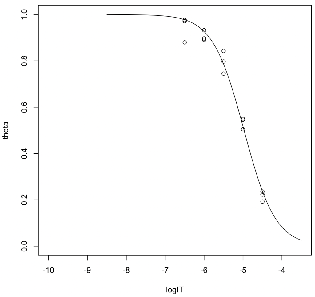
Output Highlights:
- The estimated \(\log_{10} \mathrm{IC}_{50}\) is -4.97382. Converting this to molarity yields 10,621 nM (95%CI: 9,329–12,117).
- Slope factor (\(a\)): 1.07378
Conversion to Ki
Assuming that the unlabeled ligand undergoes non-specific binding with the same partition coefficient as [3H]PDBu, we have:
$$ \mathrm{IC}_{50} = (1 + k) [I]_{50} + [RI]_{50} $$
$$ [I]_{50} = \frac{1}{1+ k} (\mathrm{IC}_{50} - [RI]_{50}) $$
Therefore, the following exact correction formula for converting \(\mathrm{IC}_{50}\) to \(K_\mathrm{i}\) is obtained:
$$ K_{\rm i} = \frac{\frac{1}{1 + k} \left[\mathrm{IC}_{50} - \left( 1 - \frac{1}{2} \frac{[L]_0}{[L]_{50}} \right)[R]_{\mathrm{T}} - \left( \frac{[L]_0}{[L]_{50}} - 1\right) \frac{[RL]_{0}}{2} \right] }{2\frac{[L]_{50}}{[L]_0} - 1 + \frac{[L]_{50}}{K_{\rm d}}} $$
In this case, since the affinity of the unlabeled ligand is weak and \(\mathrm{IC}_{50} \gg [RI]_{50}\) holds, the following approximation can be applied:
$$ [I]_{50} \simeq \frac{1}{1+ k} \mathrm{IC}_{50} $$
$$ K_{\rm i} = \frac{\frac{1}{1 + k} \mathrm{IC}_{50} }{2\frac{[L]_{50}}{[L]_0} - 1 + \frac{[L]_{50}}{K_{\rm d}}} $$
The \(K_{\rm i}\) value obtained using the exact formula was 340.6 nM (95% CI: 299.1–388.6). The \(K_{\rm i}\) value calculated with the approximation formula was 340.7 nM, demonstrating that there is no significant difference between the two.
Linear Regression via Logit Transformation (Alternative)
1) Using all five concentration levels
logIT <- c(-6.5,-6.5,-6.5,-6,-6,-6,-5.5,-5.5,-5.5,-5,-5,-5,-4.5,-4.5,-4.5)
logit <- c(1.533, 1.615, 0.865, 0.939, 0.911, 1.139, 0.465, 0.729, 0.594, 0.079, 0.085, 0.008, -0.543, -0.512, -0.623)
result_lm <- lm(logit ~ logIT)
summary(result_lm)
Output:
Call:
lm(formula = logit ~ logIT)

Residuals:
     Min       1Q   Median       3Q      Max
-0.56720 -0.04945 -0.00430  0.10460  0.24340

Coefficients:
            Estimate Std. Error t value Pr(>|t|)
(Intercept) -4.72070    0.40386  -11.69 2.86e-08 ***
logIT       -0.94660    0.07283  -13.00 7.98e-09 ***
---
Signif. codes:  0 ‘***’ 0.001 ‘**’ 0.01 ‘*’ 0.05 ‘.’ 0.1 ‘ ’ 1

Residual standard error: 0.1995 on 13 degrees of freedom
Multiple R-squared:  0.9285,	Adjusted R-squared:  0.923
F-statistic: 168.9 on 1 and 13 DF,  p-value: 7.975e-09
2) Using the three highest concentration levels
logIT_a <- c(-5.5,-5.5,-5.5,-5,-5,-5,-4.5,-4.5,-4.5)
logit_a <- c(0.465, 0.729, 0.594, 0.079, 0.085, 0.008, -0.543, -0.512, -0.623)
result_lm_a <- lm(logit_a ~ logIT_a)
summary(result_lm_a)
Output:
Call:
lm(formula = logit_a ~ logIT_a)

Residuals:
      Min        1Q    Median        3Q       Max
-0.144000 -0.023333  0.003333  0.047667  0.120000

Coefficients:
            Estimate Std. Error t value Pr(>|t|)
(Intercept)  -5.7453     0.3396  -16.92 6.18e-07 ***
logIT_a      -1.1553     0.0677  -17.07 5.82e-07 ***
---
Signif. codes:  0 ‘***’ 0.001 ‘**’ 0.01 ‘*’ 0.05 ‘.’ 0.1 ‘ ’ 1

Residual standard error: 0.08292 on 7 degrees of freedom
Multiple R-squared:  0.9765,	Adjusted R-squared:  0.9732
F-statistic: 291.2 on 1 and 7 DF,  p-value: 5.819e-07
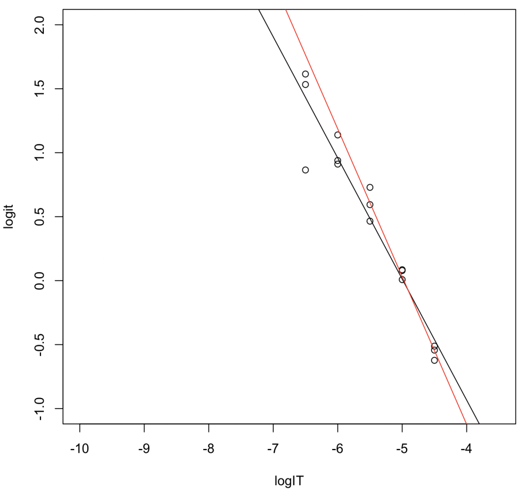
Analysis of Results
- Black Line (all five concentration levels): \(y = -0.94660x - 4.72070\). \(R^2 = 0.929\). \(\log_{10} \mathrm{IC}_{50} = -4.72070 / 0.94660 = -4.987006\). Converting to molarity gives \(\mathrm{IC}_{50} = 10,304\mbox{ nM}\).
- Red Line (the three highest concentration levels): \(y = -1.1553x - 5.7453\). \(R^2 = 0.977\). \(\log_{10} \mathrm{IC}_{50} = -5.7453 / 1.1553 = -4.972994\). Converting to molarity gives \(\mathrm{IC}_{50} = 10,642\mbox{ nM}\).
Interpretation: The \(\mathrm{IC}_{50}\) value estimated from the three-concentration levels dataset—despite having fewer data points—was closer to the results obtained via non-linear regression. This suggests that linear transformation tends to overestimate the weight of data points located at the tails of the sigmoid curve.
Using the same approximation formula from the previous section, the converted \(K_{\rm i}\) values were 330.5 nM (from the five concentration levels) and 341.3 nM (from the three concentration levels).
Tight-binding ligand
The following data obtained from a competitive binding assay using a 3H-labeled ligand (specific activity: 12.31 Ci/mmol) and an unlabeled ligand will be processed. The unit of radioactivity is dpm (disintegrations per minute; note that Bq represents disintegrations per second).
| GROUP | log10 [I]T | pellet (dpm) | supernatant (dpm) (50 μL) | |
| Total binding | — | 38985 | 10382 | |
| Total binding | — | 38931 | 10907 | |
| Total binding | — | 38495 | 9242 | |
| Total binding | — | 39034 | 10287 | |
| Nonspecific binding | — | 3629 | 14208 | |
| Nonspecific binding | — | 3448 | 13194 | |
| Unlabeled ligand (I) | -8.5 | 26327 | — | |
| Unlabeled ligand (I) | -8.5 | 26072 | — | |
| Unlabeled ligand (I) | -8.5 | 25105 | — | |
| Unlabeled ligand (I) | -8 | 13168 | — | |
| Unlabeled ligand (I) | -8 | 11354 | — | |
| Unlabeled ligand (I) | -8 | 11917 | — | |
| Unlabeled ligand (I) | -7.5 | 6314 | — | |
| Unlabeled ligand (I) | -7.5 | 6446 | — | |
| Unlabeled ligand (I) | -7.5 | 5829 | — |
Processed Data Table
| GROUP | log10 [I]T | bound (nM) | free (nM) | θ | log10 {θ/(1 − θ)} |
| Total binding (Mean) | — | 5.302 ([RL]0) | 13.05 ([L]0) | — | — |
| Unlabeled ligand (I) | -8.5 | 3.413 | — | 0.6438 | 0.257 |
| Unlabeled ligand (I) | -8.5 | 3.375 | — | 0.6365 | 0.243 |
| Unlabeled ligand (I) | -8.5 | 3.229 | — | 0.6090 | 0.193 |
| Unlabeled ligand (I) | -8 | 1.430 | — | 0.2698 | -0.432 |
| Unlabeled ligand (I) | -8 | 1.157 | — | 0.2182 | -0.554 |
| Unlabeled ligand (I) | -8 | 1.242 | — | 0.2342 | -0.515 |
| Unlabeled ligand (I) | -7.5 | 0.397 | — | 0.0750 | -1.091 |
| Unlabeled ligand (I) | -7.5 | 0.417 | — | 0.0787 | -1.068 |
| Unlabeled ligand (I) | -7.5 | 0.324 | — | 0.0612 | -1.186 |
Estimation of IC50
logIT <- c(-8.5,-8.5,-8.5,-8,-8,-8,-7.5,-7.5,-7.5)
theta <- c(0.6438,0.6365,0.6090,0.2698,0.2182,0.2342,0.0750,0.0787,0.0612)
result = nls(theta~1/(1+exp(a*log(10)*(logIT - logIC50))),start = c(logIC50=-8.5, a=1))
summary(result)
Output:
Nonlinear regression model
  model: theta ~ 1/(1 + exp(a * log(10) * (logIT - logIC50)))
   data: parent.frame()
logIC50       a
 -8.341   1.417
 residual sum-of-squares: 0.002774

Number of iterations to convergence: 5
Achieved convergence tolerance: 8.394e-06
Output Highlights:
- The estimated \(\log_{10} \mathrm{IC}_{50}\) is -8.341. Converting this to molarity yields 4.560 nM.
- Slope factor (\(a\)): 1.417
- Using the Munson–Rodbard equation, the converted \(K_\mathrm{i}\) value is 0.0586 nM.
Linear Regression via Logit Transformation (Alternative)
logIT <- c(-8.5,-8.5,-8.5,-8,-8,-8,-7.5,-7.5,-7.5)
logit = c(0.257,0.243,0.193,-0.432,-0.554,-0.515,-1.091,-1.068,-1.186)
result_lm = lm(logit ~ logIT)
summary(result_lm)
Output:
Call:
lm(formula = logit ~ logIT)

Residuals:
     Min       1Q   Median       3Q      Max
-0.09256 -0.05156  0.02944  0.04344  0.06644

Coefficients:
             Estimate Std. Error t value Pr(>|t|)
(Intercept) -11.22944    0.38820  -28.93 1.52e-08 ***
logIT        -1.34600    0.04846  -27.77 2.01e-08 ***
---
Signif. codes:  0 ‘***’ 0.001 ‘**’ 0.01 ‘*’ 0.05 ‘.’ 0.1 ‘ ’ 1

Residual standard error: 0.05935 on 7 degrees of freedom
Multiple R-squared:  0.991,	Adjusted R-squared:  0.9897
F-statistic: 771.4 on 1 and 7 DF,  p-value: 2.014e-08
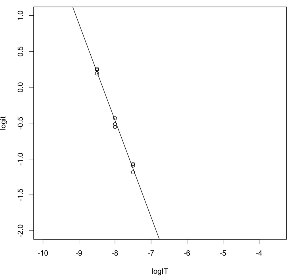
Output Highlights:
- Regression Equation: \(y = -1.34600x - 11.22944\)
- \(R^2 = 0.991\)
- \(\log_{10} \mathrm{IC}_{50} = -11.22944 / 1.34600 = -8.342823\). Converting this to molarity yields 4.541 nM.
- Using the Munson–Rodbard equation, the converted \(K_\mathrm{i}\) value is 0.0580 nM.