Using the simulated annealing method in GROMACS, a conformational search of small molecules is performed in vacuum.
This tutorial assumes that you are using a GROMACS version from the 2025 series together with AmberTools 25.
Updated on June 26, 2025.
- OS: macOS Sequoia 15.5, Chip: Apple M4, RAM: 16 GB.
- AmberTools 25
- GROMACS 2025.1
- VMD 1.9.4a57-arm64-Rev12
(Published as a static page on October 17, 2016. Converted to a blog post and updated on June 26, 2025.)
Note: The method described below performs simulations in vacuum using force field parameters optimized for aqueous environments. It is not intended for accurate simulations but rather for generating a variety of conformations. Typically, Monte Carlo methods as implemented in software like Spartan or Macromodel are used for such conformational search. This tutorial explores whether a similar goal can be achieved using the free software GROMACS. Details such as the temperature settings, heating/cooling schedule, and simulation duration for simulated annealing have not been thoroughly optimized.
Contents
Step 1: Building a small molecule
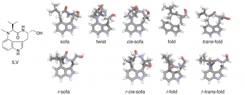
First, use Avogadro to build the 3D structure of a small molecule. In this tutorial, the example used is indolactam-V (ILV), a 9-membered ring lactam (ILV.mol2). While the GAFF force field is designed for use with the TIP3P water model, this tutorial performs calculations in vacuum, since the goal is to generate conformations by overcoming energy barriers (and vacuum calculations are also faster).
Step 2: Preparing the small molecule topology
Use Antechamber, which is included in AmberTools (freely distributed; installation instructions for macOS 15 available).
$ antechamber -fi mol2 -fo prepi -i ILV.mol2 -o ILV.prep -c bcc -at gaff2 -rn ILV
$ parmchk2 -i ILV.prep -o ILV.frcmod -f prepi -s gaff2
$ tleap
> source leaprc.gaff2
> loadamberprep ILV.prep
> loadamberparams ILV.frcmod
> mol = loadpdb NEWPDB.PDB
> saveamberparm mol ILV.prmtop ILV.inpcrd
> quit
You can run tleap by saving and executing the script shown below.tleap.in
source leaprc.gaff2
loadamberprep ILV.prep
loadamberparams ILV.frcmod
mol = loadpdb NEWPDB.PDB
saveamberparm mol ILV.prmtop ILV.inpcrd
quit
$ tleap -s -f tleap.in > tleap.out
Next, use ParmEd, also included with AmberTools, to convert the Amber-format files into GROMACS format.
Run the following script (ambergromacs.py).
import parmed as pmd
# Load AMBER format
amber = pmd.load_file('ILV.prmtop',xyz='ILV.inpcrd')
# Save a GROMACS topology and GRO files
amber.save('gromacs.top')
amber.save('gromacs.gro')
$ $AMBERHOME/miniconda/bin/python ./ambergromacs.py
This will generate gromacs.top and gromacs.gro.
Note: The topology generated by Antechamber may sometimes result in a total atomic charge that deviates from zero. In such cases, open the GROMACS .top file in a text editor and manually adjust the atomic charges to ensure the total is zero. Usually, the charge deviation is small and can be evenly distributed across all atoms.
Step 3: Running simulated annealing protocol
Preparing mdp file for a test run (sa5cycles.mdp).
sa5cycles.mdp
; Run parameters
integrator	= md		; leap-frog integrator
nsteps		= 25000		; 1 * 25000 = 25 ps; 5 cycles
dt		= 0.001		; 1 fs
; Output control
nstxout		= 100		; save coordinates every 0.2 ps
nstvout		= 100		; save velocities every 0.2 ps
nstenergy	= 100		; save energies every 0.2 ps
nstlog		= 100		; update log file every 0.2 ps
; Bond parameters
continuation	= no		; first dynamics run
constraint_algorithm = lincs	; holonomic constraints
constraints	= all-bonds	; all bonds (even heavy atom-H bonds) constrained
comm_mode       = angular
lincs_iter	= 1		; accuracy of LINCS
lincs_order	= 4		; also related to accuracy
lincs-warnangle = 90
; Neighborsearching
cutoff-scheme   = Verlet
pbc		= xyz
; Temperature coupling is on
tcoupl		= V-rescale	; modified Berendsen thermostat
tc-grps		= Other	; two coupling groups - more accurate
tau_t		= 0.1	; time constant, in ps
ref_t		= 300 	; reference temperature, one for each group, in K
; Velocity generation
; SIMULATED ANNEALING CONTROL
annealing       =  periodic
annealing_npoints  = 6
annealing_time  = 0 1 2 3 4 5
annealing_temp  = 1500 1500 1500 100 0 0
Generate .tpr file.
$ gmx editconf -f gromacs.gro -bt cubic -d 1 -o box.gro
$ gmx grompp -f sa5cycles.mdp -c box.gro -p gromacs.top -o sa_test.tpr -maxwarn 1
Run test simulation.
$ gmx mdrun -v -deffnm sa_test -ntmpi 1 -ntomp 1
Check if the temperature is changing as intended using gmx energy.
$ gmx energy -f sa_test.edr -o temperature.xvg
$ xmgrace temperature.xvg # brew install grace
Type “12 0” and enter.
Visualize temperature.xvg file.
$ xmgrace temperature.xvg
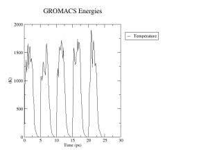
Once you have confirmed that simulated annealing has been done properly (see right figure), run 100 cycles of simulated annealing. Save both structure and energy at each cycle (see sa.mdp).
sa.mdp
; Run parameters
integrator	= md		; leap-frog integrator
nsteps		= 500000        ; 1 * 500000 = 500 ps; 100 cycles
dt		= 0.001		; 1 fs
; Output control
nstxout		= 5000		; save coordinates every 0.2 ps
nstvout		= 5000		; save velocities every 0.2 ps
nstenergy	= 5000		; save energies every 0.2 ps
nstlog		= 5000		; update log file every 0.2 ps
; Bond parameters
continuation	= no		; first dynamics run
constraint_algorithm = lincs	; holonomic constraints
constraints	= all-bonds	; all bonds (even heavy atom-H bonds) constrained
comm_mode       = angular
lincs_iter	= 1		; accuracy of LINCS
lincs_order	= 4		; also related to accuracy
lincs-warnangle = 90
; Neighborsearching
cutoff-scheme   = Verlet
pbc		= xyz
; Temperature coupling is on
tcoupl		= V-rescale	; modified Berendsen thermostat
tc-grps		= Other	; two coupling groups - more accurate
tau_t		= 0.1	; time constant, in ps
ref_t		= 300 	; reference temperature, one for each group, in K
; Velocity generation
; SIMULATED ANNEALING CONTROL
annealing       =  periodic
annealing_npoints  = 6
annealing_time  = 0 1 2 3 4 5
annealing_temp  = 1500 1500 1500 100 0 0
Caution: At sufficiently high temperatures, molecules with carbon–carbon double bonds may undergo cis–trans isomerization.
$ gmx grompp -f sa.mdp -c box.gro -p gromacs.top -o sa.tpr -maxwarn 1
$ gmx mdrun -v -deffnm sa -ntmpi 1 -ntomp 1
The calculation will finish in about 7 seconds.
Step 4: 結果の解析
Although GROMACS includes the g_cluster tool, this tutorial uses a VMD extension for clustering.
Download and extract Clustering 2.0. Copy the directory to an appropriate location and add the following line to your ~/.vmdrc file:.
menu main on
set auto_path [linsert $auto_path 0 {location of clustering plugin}]
vmd_install_extension clustering clustering "WMC PhysBio/Clustering"
Start VMD and load the trajectory from the simulated annealing run.
$ vmd sa.gro sa.trr # vmd: aliased to /Applications/VMD 1.9.4a57-arm64-Rev12.app/Contents/vmd/vmd_MACOSXARM64
Go to Extensions → Analysis → RMSD Trajectory Tool.
Change the selection from protein to resname ILV, and click the Align button to align all frames to the initial structure.
Next, go to Extensions → WMC PhysBio → Clustering to perform clustering analysis.
Set the selection to resname ILV, uncheck noh, and set num to 20.
Change the Cutoff under Use measure cluster from 1 to 0.9. Click Calculate—clusters will be color-coded and displayed at the bottom. Analyze the results visually.
Indolactam-V (ILV) exists in solution as a mixture of two stable conformers (cis-amide and trans-amide types), and both signals are observed in NMR spectra. The clusters that appeared multiple times during the simulation are as follows (conformers are classified using Itai’s nomenclature):
- Cluster 0 (23): Sofa conformer with trans-amide. Matches the NMR spectrum. This is the initial structure.
- Cluster 1 (11): Sofa conformer. Differs from Cluster 0 in the conformation of the isopropyl group at position 12.
- Cluster 2 (5): Sofa conformer. Essentially the same as Cluster 0, differing only in the conformation of the hydroxymethyl group.
- Cluster 3 (5): r–Cis-sofa conformer. Not observed in NMR.
- Cluster 4 (4): Twist conformer with cis-amide. Matches the NMR spectrum.
- Cluster 5 (2): r–Trans-fold conformer.
If stable conformers cannot be clearly identified, consider comparing energies using different force fields or molecular orbital (MO) calculations. It is also possible to use multiple conformers for docking simulations.