Contents
母集団
下の図で表わされている5つの正規母集団からサンプリングをしてみます。
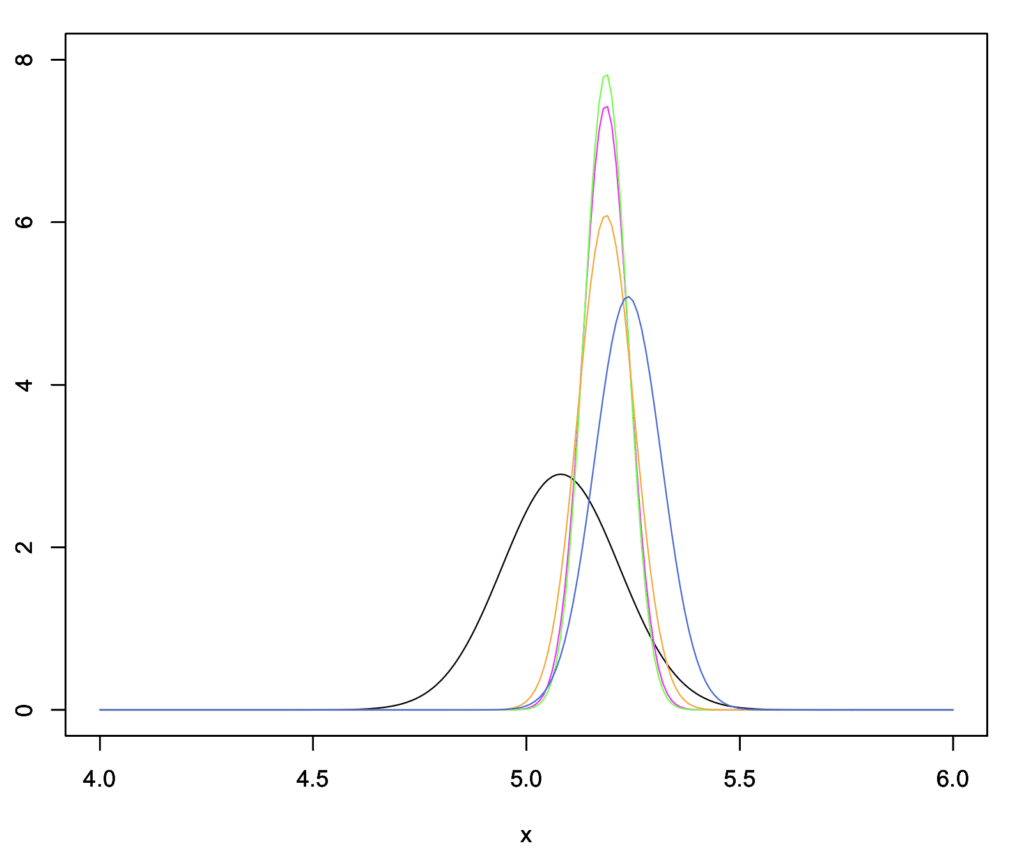
| 群 | 平均値 | 分散 | 標準偏差 |
| A | 5.080 | 0.0189 | 0.138 |
| B | 5.1859 | 0.0029 | 0.054 |
| C | 5.1861 | 0.0026 | 0.051 |
| D | 5.1864 | 0.0043 | 0.066 |
| E | 5.238 | 0.0062 | 0.078 |
群Aと群Eの母平均の差の効果量は\(\frac{|5.238295-5.080351|}{\sqrt{\frac{0.07842281^2+0.1375497^2}{2}}} \fallingdotseq 1.41\)であり、少なくともこの効果を検出したい。ランダムサンプリング(100,000回)を繰り返した時の5%水準棄却率を下の表に示します。
| 5%水準棄却率 | ||||
| n | 分散分析(等分散) | Tukey HSD検定 (群A vs. 群E) | 分散分析(不等分散) | Games–Howell法 (群A vs. 群E) |
| 2 | 0.2001 | 0.17744 | 0.13715 | –a |
| 3 | 0.32522 | 0.30633 | 0.17187 | 0.06232 |
| 4 | 0.43086 | 0.4194 | 0.22275 | 0.11431 |
| 5 | 0.52356 | 0.51794 | 0.28777 | 0.17495 |
| 6 | 0.60893 | 0.60763 | 0.35448 | 0.24316 |
| 7 | 0.67901 | 0.68453 | 0.42531 | 0.31413 |
| 8 | 0.74135 | 0.74673 | 0.49672 | 0.38871 |
| 9 | 0.79499 | 0.80356 | 0.5624 | 0.46233 |
| 10 | 0.83522 | 0.84478 | 0.62689 | 0.53158 |
| 15 | 0.95355 | 0.95965 | 0.84763 | 0.8014 |
| 20 | 0.98822 | 0.99006 | 0.94668 | 0.92978 |
等分散を仮定する検定法では\(n = 9\)、等分散を仮定しない検定法では\(n = 15\)で検出力80%に達しています。データは明らかに不等分散ですので、等分散を仮定した分散分析とTukeyのHSD法では不適切に甘く検定をしていることになります。
次に、有意水準5%で検定した時に分散分析(等分散を仮定)で有意差が出ず、TukeyのHSD検定でA群とE群の間で有意差が出る確率を10,000回のランダムサンプリングから出してみたところ、0.971%でした。
| n = 15 | Tukey \(p < 0.05\) (群A vs. 群E) | Tukey \(p \ge 0.05\) (群A vs. 群E) |
| 分散分析 (等分散を仮定) \(p < 0.05\) | 94.975% | 0.468% |
| 分散分析 (等分散を仮定) \(p \ge 0.05\) | 0.971% | 3.586% |
分散分析(等分散を仮定しない)では有意差が出ず、Games–Howell法でA群とE群の間で有意差が出る確率は2.012%でした。
| n = 15 | Games–Howell \(p < 0.05\) (群A vs. 群E) | Games–Howell \(p \ge 0.05\) (群A vs. 群E) |
| 分散分析 (等分散を仮定しない) \(p < 0.05\) | 78.11% | 6.654% |
| 分散分析 (等分散を仮定しない) \(p \ge 0.05\) | 2.012% | 13.224% |
具体的なデータの例 (n = 15)
ランダムサンプリングしたあるデータ(各群n = 15)を解析してみます。
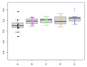
| 群 | n | 平均値 | 不偏分散 | 不偏標準偏差 |
| A | 15 | 5.1120 | 0.0193 | 0.1390 |
| B | 15 | 5.1831 | 0.0031 | 0.0560 |
| C | 15 | 5.1965 | 0.0026 | 0.0508 |
| D | 15 | 5.1984 | 0.0059 | 0.0771 |
| E | 15 | 5.2409 | 0.0073 | 0.0856 |
#R内での上のデータの生成
N=15
set.seed(-6152847)
a <- rnorm(N, mean=5.080351, sd=0.1375497)
set.seed(3448258)
b <- rnorm(N, mean=5.185921, sd=0.05358547)
set.seed(-9846648)
c <- rnorm(N, mean=5.186056, sd=0.05089308)
set.seed(-1377657)
d <- rnorm(N, mean=5.186409, sd=0.06550713)
set.seed(7612155)
e <- rnorm(N, mean=5.238295, sd=0.07842281)
set.seed(NULL)
value <- c(a, b, c, d, e)
group <- factor(c(rep("A", N), rep("B", N), rep("C", N), rep("D", N), rep("E", N)))
df <- data.frame(group, value)
Rを使った解析
すべて有意水準5%で検定します。
Welchのt検定を使った対比較
Welchのt検定
> pairwise.t.test(value, group, pool.sd=FALSE, p.adj="none")

	Pairwise comparisons using t tests with non-pooled SD

data:  value and group

  A      B      C      D
B 0.0826 -      -      -
C 0.0404 0.4960 -      -
D 0.0470 0.5377 0.9369 -
E 0.0055 0.0383 0.0974 0.1642

P value adjustment method: none
群A vs. 群Eが\(p = 0.0055\)なので、有意水準5%で余裕で帰無仮説を棄却できそうですが、検定の多重性が考慮されていません。
分散分析(等分散を仮定しない)
別記事。
> oneway.test(value ~ group, var.equal=FALSE)

	One-way analysis of means (not assuming equal variances)

data:  value and group
F = 2.4529, num df = 4.000, denom df = 34.283, p-value = 0.06439
\(p = 0.06439 \ge 0.05\)なので、「全ての群の母平均に差はない」という帰無仮説は保留されました。
Games–Howell法(等分散を仮定しない)で対比較
tukey関数はShigenobu AOKI (2009-08-03) テューキーの方法による多重比較から読み込みました。
> tukey(value, group, method="Games-Howell")
$result1
        n     Mean    Variance
Group1 15 5.112008 0.019333908
Group2 15 5.183060 0.003138345
Group3 15 5.196527 0.002576593
Group4 15 5.198433 0.005945748
Group5 15 5.240933 0.007322983

$Games.Howell
             t       df          p
1:2 1.83570268 18.42837 0.38416403
1:3 2.21144418 17.66639 0.22075686
1:4 2.10523223 21.86683 0.25336137
1:5 3.05828117 23.27480 0.03988291
2:3 0.68992946 27.73205 0.95700608
2:4 0.62466841 25.55888 0.96971279
2:5 2.19140328 24.13776 0.21669158
3:4 0.07995019 24.21543 0.99999001
3:5 1.72851490 22.76652 0.43735024
4:5 1.42894943 27.70156 0.61494734
群A vs. 群Eで\(p = 0.03988291 < 0.05\)なので、「群Aと群Eの母平均に差はない」という帰無仮説は棄却されました。
Welchのt検定(等分散を仮定しない)+ Bonferroni補正
> pairwise.t.test(value, group, pool.sd=FALSE, p.adj="bonferroni")

	Pairwise comparisons using t tests with non-pooled SD

data:  value and group

  A     B     C     D
B 0.826 -     -     -
C 0.404 1.000 -     -
D 0.470 1.000 1.000 -
E 0.055 0.383 0.974 1.000

P value adjustment method: bonferroni
Bonferroniの補正では検定の数\(m = 10\)で有意水準αを割るので、α = 0.05/10 = 0.005で検定します。上の出力では計算されたp値が10倍されています。群A vs. 群Eで\(p = 0.055 \ge 0.05\)なので、「群Aと群Eの母平均に差はない」という帰無仮説は保留されました。
Welchのt検定(等分散を仮定しない)+ Holm-Bonferroni補正
> pairwise.t.test(value, group, pool.sd=FALSE, p.adj="holm")

	Pairwise comparisons using t tests with non-pooled SD

data:  value and group

  A     B     C     D
B 0.496 -     -     -
C 0.345 1.000 -     -
D 0.345 1.000 1.000 -
E 0.055 0.345 0.496 0.657

P value adjustment method: holm
Holm–Bonferroni補正はステップダウン法と呼ばれる方法の一つで、検定の数\(m = 10\)とすると一番小さなp値を有意水準\(\alpha/m\)で検定して、次に小さなp値を有意水準\(\alpha/(m-1)\)で検定して、を繰り返して棄却されなかったところで打ち切ります。上の出力では割るのではなくp値が整数倍されています。今回は結果としてBonferroni補正と同じで、群A vs. 群Eで\(p = 0.055 \ge 0.05\)なので帰無仮説は保留されました。
不適切な検定法: 分散分析(等分散を仮定)
> oneway.test(value ~ group, var.equal=TRUE)

	One-way analysis of means

data:  value and group
F = 4.2896, num df = 4, denom df = 70, p-value = 0.00367
\(p = 0.00367 < 0.05\)なので、「全ての群の母平均に差はない」という帰無仮説は棄却されました。しかし、p値がWelchのt検定のp値よりも小さいです。次にTukeyのHSD法で多重比較を行ってみます。
不適切な検定法: TukeyのHSD検定(等分散を仮定)で対比較
> TukeyHSD(aov(value ~ group))
  Tukey multiple comparisons of means
    95% family-wise confidence level

Fit: aov(formula = value ~ group)

$group
           diff          lwr        upr     p adj
B-A 0.071052607 -0.018456070 0.16056128 0.1834851
C-A 0.084519419 -0.004989258 0.17402810 0.0732990
D-A 0.086425114 -0.003083563 0.17593379 0.0634977
E-A 0.128924820  0.039416143 0.21843350 0.0012702
C-B 0.013466812 -0.076041866 0.10297549 0.9932698
D-B 0.015372507 -0.074136171 0.10488118 0.9888662
E-B 0.057872213 -0.031636465 0.14738089 0.3758897
D-C 0.001905695 -0.087602983 0.09141437 0.9999971
E-C 0.044405401 -0.045103276 0.13391408 0.6365763
E-D 0.042499706 -0.047008971 0.13200838 0.6738995
群A vs. 群Eで\(p = 0.0012702 < 0.05\)なので、「群Aと群Eの母平均に差はない」という帰無仮説は棄却されました。なぜWelchのt検定でのA群 vs. E群のp値 (0.0055) の約5分の1と極端に小さいp値が出るかといえば、Tukey法の検定統計量q
$$q = \frac{|\bar{X_A} – \bar{X_B}|}{\sqrt{\frac{S_R^2}{2}\left(\frac{1}{n_A}+\frac{1}{n_B}\right)}} $$
を計算する際に誤差分散\(s_R^2\)(各群の不偏分散の平均値)を使用するためです。A群とE群の分散は大きいのに、B、C、D群の分散が小さいので、結果としてp値が非常に小さくなってしまいました。このように等分散を仮定した分散分析とTukeyのHSD検定を、nが小さく不等分散のデータに対して使うべきでないことが分かりました。はじめから等分散を仮定しないGames–Howell法を使用しましょう。
(了)