GROMACSのSimulated annealing methodを使用して,真空中での低分子化合物の配座探索を行う.
This tutorial assumes you are using a GROMACS version in the 2020 series with AmberTools 19.
Updated on March 12, 2020.環境: macOS Mojave 10.14.6, 3.3 GHz Intel Core i5, メモリ8 GB.
注意: 以下の方法は水中でのシミュレーションに最適化された力場パラメータを使って真空中でのシミュレーションを行うもので,正確なシミュレーションではなく様々な配座を発生させることを目的としています.本来こういった目的にはSpartanやMacromodelで使われるモンテカルロ法がありますが,無償のGromacsで似たことをできないかとやってみたものです.Simulated annealingの温度の値や上げ方,下げ方,時間については検討していません.
Contents
Step 1: Building a small molecule
まず,Avogadroを使用して低分子の3次元構造を作成する.このチュートリアルでは,例として9員環ラクタムであるindolactam-V (ILV) を取り上げる (ILV.mol2).GAFF力場はTIP3P水モデル中での使用が適切だが,今回はエネルギー障壁を超えてコンホメーションを生成することが目的なので真空中で計算する (計算も早く終わる).
Step 2: Preparing the small molecule topology
以前は以下のようにACPYPEを使用していました.
$ acpype -i ILV.mol2素のACPYPEだとAMBER GAFF力場 (Version 1.81, May 2017) によってtopology fileが作成される.最新のGAFF2力場 (version 2.11, May 2016) を使用したい場合は,以下のようにantechamberを使用する.
$ antechamber -fi mol2 -fo prepi -i ILV.mol2 -o ILV.prep -c bcc -at gaff2 -rn ILV
$ parmchk2 -i ILV.prep -o ILV.frcmod -f prepi -s gaff2
$ tleap
> source leaprc.gaff2
> loadamberprep ILV.prep
> loadamberparams ILV.frcmod
> mol = loadpdb NEWPDB.PDB
> saveamberparm mol ILV.prmtop ILV.inpcrd
> quit
tleapの実行は上記のスクリプトを保存して実行してもよい.
tleap.in
source leaprc.gaff2
loadamberprep ILV.prep
loadamberparams ILV.frcmod
mol = loadpdb NEWPDB.PDB
saveamberparm mol ILV.prmtop ILV.inpcrd
quit
$ tleap -s -f tleap.in > tleap.outAmberTools付属のParmEdを使用して,Amber形式のファイルをGROMACS形式へ変換する.
以下のscript (ambergromacs.py) を実行する.
import parmed as pmd
# Load AMBER format
amber = pmd.load_file('ILV.prmtop',xyz='ILV.inpcrd')
# Save a GROMACS topology and GRO files
amber.save('gromacs.top')
amber.save('gromacs.gro')
$ python ./ambergromacs.pygromacs.topとgromacs.groが書き出されます.
今まで通り,ACPYPEを使用しても同じです (電荷の書き出しにバグあり).
$ acpype -p ILV.prmtop -x ILV.inpcrd
とするとILV_GMX.gro, ILV_GMX.topが生成される.ACPYPEを使用するとGROMACS用のmdpファイルも生成してくれて便利ではある.
antechamberで生成したトポロジーでは,原子電荷の総和が0からずれる時がある.そういった場合は,GROMACSのtopファイルをテキストエディタで開き,原子電荷の総和が0になるように修正する.
Step 3: Running simulated annealing protocol
Preparing mdp file for a test run (sa5cycles.mdp).
sa5cycles.mdp
title		= ILV simulated annealing in vacuo
; Run parameters
integrator	= md		; leap-frog integrator
nsteps		= 25000		; 1 * 25000 = 25 ps; 5 cycles
dt		= 0.001		; 1 fs
; Output control
nstxout		= 100		; save coordinates every 0.2 ps
nstvout		= 100		; save velocities every 0.2 ps
nstenergy	= 100		; save energies every 0.2 ps
nstlog		= 100		; update log file every 0.2 ps
; Bond parameters
continuation	= no		; first dynamics run
constraint_algorithm = lincs	; holonomic constraints
constraints	= all-bonds	; all bonds (even heavy atom-H bonds) constrained
comm_mode       = angular
lincs_iter	= 1		; accuracy of LINCS
lincs_order	= 4		; also related to accuracy
lincs-warnangle = 90
; Neighborsearching
cutoff-scheme   = Verlet
pbc		= xyz
; Temperature coupling is on
tcoupl		= V-rescale	; modified Berendsen thermostat
tc-grps		= Other	; two coupling groups - more accurate
tau_t		= 0.1	; time constant, in ps
ref_t		= 300 	; reference temperature, one for each group, in K
; Velocity generation
; SIMULATED ANNEALING CONTROL
annealing       =  periodic
annealing_npoints  = 6
annealing_time  = 0 1 2 3 4 5
annealing_temp  = 1500 1500 1500 100 0 0
Generate .tpr file.
$ gmx editconf -f gromacs.gro -bt cubic -d 1 -o box.gro
$ gmx grompp -f sa5cycles.mdp -c box.gro -p gromacs.top -o sa_test.tpr -maxwarn 1
Run test simulation.
$ gmx mdrun -v -deffnm sa_test温度が設定通り変化しているかをgmx energyで確認.
$ gmx energy -f sa_test.edr -o temperature.xvgType “12 0” and enter.
Visualize temperature.xvg file.
$ xmgrace temperature.xvg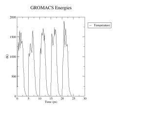 Simulated annealingが実行できていると確認できた (右図) ので100サイクルのsimulated annealingを実行する.各サイクル毎に構造およびエネルギーを保存する (sa.mdp).
sa.mdp
title		= ILV simulated annealing in vacuo
; Run parameters
integrator	= md		; leap-frog integrator
nsteps		= 500000        ; 1 * 500000 = 500 ps; 100 cycles
dt		= 0.001		; 1 fs
; Output control
nstxout		= 5000		; save coordinates every 0.2 ps
nstvout		= 5000		; save velocities every 0.2 ps
nstenergy	= 5000		; save energies every 0.2 ps
nstlog		= 5000		; update log file every 0.2 ps
; Bond parameters
continuation	= no		; first dynamics run
constraint_algorithm = lincs	; holonomic constraints
constraints	= all-bonds	; all bonds (even heavy atom-H bonds) constrained
comm_mode       = angular
lincs_iter	= 1		; accuracy of LINCS
lincs_order	= 4		; also related to accuracy
lincs-warnangle = 90
; Neighborsearching
cutoff-scheme   = Verlet
pbc		= xyz
; Temperature coupling is on
tcoupl		= V-rescale	; modified Berendsen thermostat
tc-grps		= Other	; two coupling groups - more accurate
tau_t		= 0.1	; time constant, in ps
ref_t		= 300 	; reference temperature, one for each group, in K
; Velocity generation
; SIMULATED ANNEALING CONTROL
annealing       =  periodic
annealing_npoints  = 6
annealing_time  = 0 1 2 3 4 5
annealing_temp  = 1500 1500 1500 100 0 0
ある程度高い温度の場合,炭素-炭素二重結合を持つ分子ではシス-トランス異性化が起こってしまうので注意すること.
$ gmx grompp -f sa.mdp -c box.gro -p gromacs.top -o sa.tpr -maxwarn 1
$ gmx mdrun -v -deffnm sa
12秒程で計算終了.
Step 4: 結果の解析
Gromacs付属のg_clusterも使用できるが,VMDのextensionを使用する (clustering).
Clustering 2.0をダウンロードして解凍する.適当な場所にdirectoryをコピー.~/.vmdrcに以下のように書いておく.
menu main on
set auto_path [linsert $auto_path 0 {clusteringフォルダの場所}]
vmd_install_extension clustering clustering "WMC PhysBio/Clustering"
VMDを起動して先程のsimulated annealingのtrajectoryを表示.
$ vmd sa.gro sa.trrExtensions→Analysis→RMSD Trajectory Tool
selectionをproteinからresname LIGに書き換え,Alignボタンをクリックすると初期構造を基準に分子の向きが揃う.
Extensions→WMC PhysBio→Clustering を起動してクラスター解析を行う.
selectionをresname LIGに書き換える.nohのチェックをはずす.
Use measure clusterのCutoffを1から0.9に変更して,Calculateボタンをクリックすると下部にクラスターが色分けされて表示される.結果を目で見て解析する.
ILVは溶液中で2つの安定コンホマー(cis-amide型とtrans-amide型)の平衡混合物として存在しており,NMRではそれぞれのコンホマーのシグナルが観測される.今回のシミュレーションに複数回現われたコンホメーションのクラスターは以下の通り (Conformers are classified on the basis of Itai’s nomenclature).
- Cluster 0 (23): Sofa conformer with trans-amide. NMRスペクトルと一致する.※初期構造
- Cluster 1 (11): Sofa conformer. Cluster 0とは12位のイソプロピル基の配座が異なる.
- Cluster 2 (5): Sofa conformer. Cluster 0とはヒドロキシメチル基の配座が異なるのみで実質同じ.
- Cluster 3 (5): r–Cis-sofa conformer. NMRでは観測されない.
- Cluster 4 (4): Twist conformer with cis-amide. NMRスペクトルと一致する
- Cluter 5 (2): r–Trans-fold conformer.
安定コンホマーが同定できない場合は,他の力場やMO計算でエネルギー比較を行う.また,複数のコンホマーをDocking simulationに使用してもよい.