研究室内メモ
環境: CentOS 7.
GROMACS 2019.4, PLUMED 2.6.0, GCC 6.3.1, OpenMPI 4.0.2, AmberTools 19.
参考サイト: Using Hamiltonian replica exchange with GROMACS – www.plumed.org
参考文献: Giovanni, B. Hamiltonian replica exchange in GROMACS: a flexible implementation.
Mol. Phys. 2014, 112, 379–384. DOI: 10.1080/00268976.2013.824126
Wang, L.; Friesner, R. A.; Berne, B. J. Replica Exchange with Solute Scaling: A More Efficient Version of Replica Exchange with Solute Tempering (REST2).
J. Phys. Chem. B 2011, 115, 9431-9438. DOI:10.1021/jp204407d
Contents
復習: 温度レプリカ交換MD
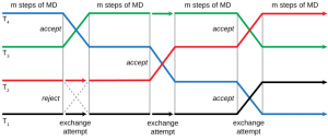
Temperature Replica Exchange Molecular Dynamics(温度レプリカ交換MD、T-REMD)法では、シミュレーションのlocal minimum間の障壁を超えて効率的にサンプリングを行うため(小分子とタンパク質の結合様式だったり、タンパク質/ペプチドのコンホメーションだったり)、温度が異なるレプリカを複数用意してメトロポリス=ヘイスティングズ基準(Metropolis–Hastings criterion。確率は下の式で計算される)に従ってレプリカの座標の交換を試行します。
\( P(1↔2)=min\left(1, \exp \left[\left(\frac{1}{k_BT_1}−\frac{1}{k_BT_2}\right)(U_1−U_2)\right]\right)\)
minは小さい方を取る関数なので、状態1の方が温度が低いとして、状態1の瞬間的なポテンシャルエネルギー(\(U_1\))が状態2のエネルギー(\(U_2\))以上の場合は(\(U_1 \geq U_2\))必ず交換が行われ(確率1= 100%)、状態1の方が低ければエネルギー差に応じて指数関数的に小さくなる確率で交換されます。
圧力制御をしている場合の交換確率は、
\( P(1↔2)=min\left(1, \exp \left[\left(\frac{1}{k_BT_1}−\frac{1}{k_BT_2}\right)(U_1−U_2) + \left(\frac{P_1}{k_BT_1} – \frac{P_2}{k_BT_2}\right) (V_1 – V_2)\right]\right)\)
となりますが、ほとんどの場合体積Vの差が小さいので第2項は無視できる。
Gromacs(MPIを有効、”build_mdrun_only” オプションをonにしてmake installしたmdrun_mpiを使用)では、例えば1から4の数字の4つのディレクトリにそれぞれファイル名testrun.tprの実行ファイルが用意されているとすると
$ mpirun -np 4 --host localhost:4 mdrun_mpi -deffnm testrun -multidir [1234] -replex 500全てのシミュレーションの温度が同じであれば、100%近く交換が起こるはずです。一般に交換受容確率は0.2程度が望ましいそうです。各設定温度はTemperature generator for REMD-simulationsで計算してくれます。ただしこのサイトに入力した確率には実際には必ずしもならないので、短いシミュレーションを走らせて交換確率を確認し、何度か調整を行う必要があるでしょう。
1つのレプリカに着目すると、異なる温度をランダムウォーク(酔歩)してそれによってエネルギー障壁を超えるので、Simulated Annealing(擬似焼きなまし)法と類似しています(レプリカ交換の場合はアニリーングではなくテンパリング〈tempering、焼きもどし〉と呼ばれる)。複数のテンパリングを同時に行うため、T-REMDはParallel Tempering(平行焼きもどし)と呼ばれます。Simulated Annealing法とREMD法ではREMDの方が計算コストがかなり高くなりますが、T-REMDの利点は、それぞれの温度でアンサンブル(統計集団)に一致するトラジェクトリを生成する点です(原子の座標を交換するので構造は途中で飛んでいる)。
ハミルトニアンレプリカ交換法
解説・PLUMEDのインストール
Hamiltonian Replica Exchange (HREX) 法は温度ではなく力場のパラメータが異なるシミュレーションを複数並列実行して、それらの間で交換を行う方法です。溶質と水のパラメータを段階的に弱めたレプリカを使うReplica Exchange with Solute Scaling(REST2)は、T-REMDに比べて少ないレプリカ数で効率的にコンホメーションのサンプリングができることが示されています。
※水の温度は冷たいままで、溶質の温度だけ上げたReplica Exchange with Solute Temperingシミュレーションが “REST” と呼ばれるのに対して、”Hamiltonian” Replica Exchange with Solute Scalingは “REST2” と呼ばれる。
Gromacsには2つの状態の自由エネルギー差を計算するためのBAR(Bennett Acceptance Ratio、ベネット受容比)法が実装されていて、その時は溶質(小分子やタンパク質)と系とのクーロン相互作用やファンデルワールス相互作用を段階的に消去していきます。これを使って、例えばリガンドと周囲との相互作用を弱めたレプリカを作ることで、エネルギー障壁を超えた状態間の遷移を容易にします。ただしとても遅い(後述)。
別の方法として、PLUMEDプログラムとPLUMEDでパッチを当てたGROMACSを使用する方法があります。インストール法などはInstallation – www.plumed.orgに詳しく解説してあります。
$ source /usr/local/gromacs/2019.4_plumed/bin/GMXRC
パッチを当ててビルドしたGROMACSはHREX法のための “mdrun -hrex” オプションが使えるようになっているはずです(gmx_mpi mdrun -hで確認)。
準備
構造ファイルの作成と平衡化
AMBER Tutorial A19を参考にAmberを使ってalanineを作る。
$ source /usr/local/amber18//amber.sh
$ tleap
> source leaprc.protein.ff03ua
> m = sequence { ACE ALA NME }
> savepdb m diala.pdb
> quit
$ gmx_mpi pdb2gmx -f diala.pdb -o conf.gro -ignh
> 1 [enter]
> 1 [enter]
$ gmx_mpi editconf -f conf.gro -o box.gro -bt cubic -d 1
$ gmx_mpi solvate -cp box.gro -p topol.top -o solv.gro
アミノ酸の原子数22、水分子数752。
必要なファイルの中身:
minim.mdp
; minim.mdp - used as input into grompp to generate em.tpr
; Parameters describing what to do, when to stop and what to save
integrator  = steep         ; Algorithm (steep = steepest descent minimization)
emtol       = 1000.0        ; Stop minimization when the maximum force < 1000.0 kJ/mol/nm
emstep      = 0.01          ; Minimization step size
nsteps      = 50000         ; Maximum number of (minimization) steps to perform

; Parameters describing how to find the neighbors of each atom and how to calculate the interactions
nstlist         = 1         ; Frequency to update the neighbor list and long range forces
cutoff-scheme   = Verlet    ; Buffered neighbor searching
ns_type         = grid      ; Method to determine neighbor list (simple, grid)
coulombtype     = PME       ; Treatment of long range electrostatic interactions
rcoulomb        = 1.0       ; Short-range electrostatic cut-off
rvdw            = 1.0       ; Short-range Van der Waals cut-off
pbc             = xyz       ; Periodic Boundary Conditions in all 3 dimensions
nvt.mdp
define      = -DPOSRES; position restrain the protein
; Run parameters
integrator  = md        ; leap-frog integrator
nsteps      = 50000     ; 2 * 50000 = 100 ps
dt          = 0.002     ; 2 fs
; Output control
nstxout     = 5000       ; save coordinates every 1.0 ps
nstvout     = 5000       ; save velocities every 1.0 ps
nstenergy   = 5000       ; save energies every 1.0 ps
nstlog      = 5000       ; update log file every 1.0 ps
nstxtcout     = 5000
;energygrps  = Protein
; Bond parameters
continuation    = no           ; first dynamics run
constraint_algorithm = lincs    ; holonomic constraints
constraints     = h-bonds     ; all bonds (even heavy atom-H bonds) constrained
lincs_iter      = 1             ; accuracy of LINCS
lincs_order     = 4             ; also related to accuracy
; Neighborsearching
cutoff-scheme   = Verlet
;vdwtype =cutoff
;vdw-modifier = force-switch
rlist =1
rcoulomb        = 1       ; short-range electrostatic cutoff (in nm)
rvdw            = 1       ; short-range van der Waals cutoff (in nm)
;rvdw-switch =1.0
; Electrostatics
coulombtype     = PME       ; Particle Mesh Ewald for long-range electrostatics
pme_order       = 4         ; cubic interpolation
fourierspacing  = 0.16      ; grid spacing for FFT
; Temperature coupling
tcoupl      = V-rescale                     ; modified Berendsen thermostat
tc-grps     = Protein Water    ; two coupling groups - more accurate
tau_t       = 0.1   0.1                     ; time constant, in ps
ref_t       = 310   310                    ; reference temperature, one for each group, in K
;refcoord_scaling    = com
; Periodic boundary conditions
pbc         = xyz       ; 3-D PBC
; Dispersion correction
DispCorr    = EnerPres  ; account for cut-off vdW scheme
; Velocity generation
gen_vel     = yes        ; velocity generation off after NVT
npt.mdp
define                  = -DPOSRES  ; position restrain the protein
; Run parameters
integrator              = md        ; leap-frog integrator
nsteps                  = 50000     ; 2 * 50000 = 100 ps
dt                      = 0.002     ; 2 fs
; Output control
nstxout                 = 500       ; save coordinates every 1.0 ps
nstvout                 = 500       ; save velocities every 1.0 ps
nstenergy               = 500       ; save energies every 1.0 ps
nstlog                  = 500       ; update log file every 1.0 ps
; Bond parameters
continuation            = yes       ; Restarting after NVT
constraint_algorithm    = lincs     ; holonomic constraints
constraints             = h-bonds   ; bonds involving H are constrained
lincs_iter              = 1         ; accuracy of LINCS
lincs_order             = 4         ; also related to accuracy
; Nonbonded settings
cutoff-scheme           = Verlet    ; Buffered neighbor searching
ns_type                 = grid      ; search neighboring grid cells
nstlist                 = 10        ; 20 fs, largely irrelevant with Verlet scheme
rcoulomb                = 1.0       ; short-range electrostatic cutoff (in nm)
rvdw                    = 1.0       ; short-range van der Waals cutoff (in nm)
DispCorr                = EnerPres  ; account for cut-off vdW scheme
; Electrostatics
coulombtype             = PME       ; Particle Mesh Ewald for long-range electrostatics
pme_order               = 4         ; cubic interpolation
fourierspacing          = 0.16      ; grid spacing for FFT
; Temperature coupling is on
tcoupl                  = V-rescale             ; modified Berendsen thermostat
tc-grps                 = Protein Water   ; two coupling groups - more accurate
tau_t                   = 0.1     0.1           ; time constant, in ps
ref_t                   = 310     310           ; reference temperature, one for each group, in K
; Pressure coupling is on
pcoupl                  = Parrinello-Rahman     ; Pressure coupling on in NPT
pcoupltype              = isotropic             ; uniform scaling of box vectors
tau_p                   = 2.0                   ; time constant, in ps
ref_p                   = 1.0                   ; reference pressure, in bar
compressibility         = 4.5e-5                ; isothermal compressibility of water, bar^-1
refcoord_scaling        = com
; Periodic boundary conditions
pbc                     = xyz       ; 3-D PBC
; Velocity generation
gen_vel                 = no        ; Velocity generation is off
hrex.mdp
define                  =
; Run parameters
integrator              = md        ; leap-frog integrator
nsteps                  = 500000     ; 2 * 500000 = 1000 ps
dt                      = 0.002     ; 2 fs
; Output control
nstxout                 = 500       ; save coordinates every 1.0 ps
nstvout                 = 500       ; save velocities every 1.0 ps
nstenergy               = 500       ; save energies every 1.0 ps
nstlog                  = 500       ; update log file every 1.0 ps
; Bond parameters
continuation            = yes       ; Restarting after NVT
constraint_algorithm    = lincs     ; holonomic constraints
constraints             = h-bonds   ; bonds involving H are constrained
lincs_iter              = 1         ; accuracy of LINCS
lincs_order             = 4         ; also related to accuracy
; Nonbonded settings
cutoff-scheme           = Verlet    ; Buffered neighbor searching
ns_type                 = grid      ; search neighboring grid cells
nstlist                 = 10        ; 20 fs, largely irrelevant with Verlet scheme
rcoulomb                = 1.0       ; short-range electrostatic cutoff (in nm)
rvdw                    = 1.0       ; short-range van der Waals cutoff (in nm)
DispCorr                = EnerPres  ; account for cut-off vdW scheme
; Electrostatics
coulombtype             = PME       ; Particle Mesh Ewald for long-range electrostatics
pme_order               = 4         ; cubic interpolation
fourierspacing          = 0.16      ; grid spacing for FFT
; Temperature coupling is on
tcoupl                  = V-rescale             ; modified Berendsen thermostat
tc-grps                 = Protein Water   ; two coupling groups - more accurate
tau_t                   = 0.1     0.1           ; time constant, in ps
ref_t                   = 310     310           ; reference temperature, one for each group, in K
; Pressure coupling is on
pcoupl                  = Parrinello-Rahman     ; Pressure coupling on in NPT
pcoupltype              = isotropic             ; uniform scaling of box vectors
tau_p                   = 2.0                   ; time constant, in ps
ref_p                   = 1.0                   ; reference pressure, in bar
compressibility         = 4.5e-5                ; isothermal compressibility of water, bar^-1
refcoord_scaling        = com
; Periodic boundary conditions
pbc                     = xyz       ; 3-D PBC
; Velocity generation
gen_vel                 = no        ; Velocity generation is off
equilibration.sh
#!/bin/bash
source /usr/local/gromacs/2019.4_plumed/bin/GMXRC
gmx_mpi grompp -f minim.mdp -c solv.gro -o minim
gmx_mpi mdrun -deffnm minim
gmx_mpi grompp -f nvt.mdp -c minim.gro -r minim.gro -o nvt
gmx_mpi mdrun -deffnm nvt
gmx_mpi grompp -f npt.mdp -c nvt.gro -r nvt.gro -t nvt.cpt -o npt
gmx_mpi mdrun -deffnm npt
$ sh ./equilibration.shHREX用トポロジーの作成
Gromacsのトポロジーファイルは大抵 “#include ~~.itp” などと外部ファイルを読み込んいる箇所がありますが、plumedで処理するためには全てのパラメータが書き込まれたトポロジーファイルが必要です。これは、grompp -pp オプションで生成することができます(processed.topファイルが出力される)。
$ gmx_mpi grompp -f minim.mdp -c npt.gro -pp
出力されたprocessed.topの中で力場パラメータをスケーリングしたい分子(水中のシミュレーションなら大抵は溶質)のatom typeの後ろにアンダーバーを付加します(参考: https://www.plumed.org/doc-v2.5/user-doc/html/hrex.html)。
[ moleculetype ]
; Name            nrexcl
Protein             3

[ atoms ]
;   nr       type  resnr residue  atom   cgnr     charge       mass  typeB    chargeB      massB
; residue   1 ACE rtp ACE  q  0.0
     1         CT_      1    ACE    CH3      1  -0.190264      12.01
     2         HC_      1    ACE   HH31      2    0.07601      1.008
     3         HC_      1    ACE   HH32      3   0.076011      1.008
     4         HC_      1    ACE   HH33      4    0.07601      1.008
     5          C_      1    ACE      C      5   0.512403      12.01
Position restraintの情報も全てインクルードされているので削除します。
次に、以下のscript (scaling.py) を実行します。Python wrapperがインストール済みの場合は”import plumed”で使えます。
#! /usr/bin/env python3
import math, os, glob, subprocess

# レプリカの数
nrep = 4
# "有効" 温度範囲
tmin = 310
tmax = 1200

# build  geometric progression
temp_list = [ tmin * math.exp(i * math.log( tmax / tmin ) / ( nrep - 1 )) for i in range( nrep )]
lambda_list = [ temp_list[0] / temp_list[i] for i in range( nrep )]
print("temperature :", temp_list)
print("lambda :", lambda_list)

# 不要なファイルの削除
files = glob.glob( "./#*" )
files += glob.glob( "./topol*" )

for f in files:
    os.remove( f )

for i in range( nrep ):
    command1 = ["mkdir", "replica"+str(i)]
    subprocess.call( command1 )
    # lambdaの値をT[0]/T[i] として選ぶ。
    # 高い温度は低いlambda値に相当する。
    lambdavalue = temp_list[0] / temp_list[i]
    # トポロジーの処理
    # 結果は "diff topol0.top topol1.top" で確認できる。
    command2 = [ "plumed", "partial_tempering", str( lambdavalue ), "<", "processed.top", ">", "topol"+str(i)+".top" ]
    subprocess.call( command2 )
    command3 = [ "mv",  "topol"+str(i)+".top", "./replica"+str( i )]
    subprocess.call( command3 )

    # tprファイルの準備
    # 溶質が電荷を持っていた場合、部分電荷をスケーリングしていくとシミュレーション系の電荷が0ではなくなり警告が出るので -maxwarn 1 で回避する。
    command4 = [ "gmx_mpi", "grompp", "-maxwarn", "1", "-o", "replica"+str( i )+"/hrex.tpr", "-f", "hrex.mdp", "-c", "npt.gro", "-p", "replica"+str( i )+"/topol"+str(i)+".top" ]
    subprocess.call( command4 )
    command5 = [ "touch",  "replica"+str( i )+"/hrex.dat"] #空ファイルの作成
    subprocess.call( command5 )
$ python3 ./scaling.pyREST2シミュレーションの実行(PLUMED、1 ns)
$ mpirun -np 4 gmx_mpi mdrun -deffnm hrex -ntomp 1 -multidir replica{0..3} -replex 500 -hrex -plumed hrex.dat -pin on
Lambdaの値: [1.0, 0.532, 0.353, 0.258]。
ログファイルを見ると(replica*/hrex.log)、レプリカの交換受容確率が均一ではなく、「高温」側にいくほど高くなってしまっていた。
Repl  average number of exchanges:
Repl     0    1    2    3
Repl      .13  .21  .33
スケーリングを
lambda : [1.0, 0.706, 0.446, 0.258]
に調整したところ、
Repl  average number of exchanges:
Repl     0    1    2    3
Repl      .26  .21  .21
となった。交換受容確率は20%程度が適切とのこと(参考: 温度レプリカ交換分子動力学法についての Q&A(PDFファイル))なので概ね良好と言える。
Performanceは120.127 ns/dayだった。
GROMACS単独の機能を使ったREST2シミュレーションの実行(100 ps)
参考: Free energy of solvation tutorial – gromacs.org
run.mdp
; using sd integrator with 50000 time steps (100 ps)
integrator = sd ; stochastic (velocity Langevin) dynamics integrator。ランジュバン動力学では温度制御を行えるので、tcouplパラメータは無視される。
nsteps = 50000
dt = 0.002
nstenergy = 1000
nstlog = 5000
; cut-offs at 1.0nm
cutoff-scheme = Verlet
rlist = 1.0
dispcorr = EnerPres
vdw-type = pme
rvdw = 1.0
; Coulomb interactions
coulombtype = pme
rcoulomb = 1.0
fourierspacing = 0.12
; Constraints
constraints = all-bonds
; set temperature to 310K
; tcoupl = v-rescale ; 必要ない
tc-grps = system
tau-t = 0.2
ref-t = 310
; set pressure to 1 bar with a thermostat that gives a correct
; thermodynamic ensemble
pcoupl = parrinello-rahman
ref-p = 1
compressibility = 4.5e-5
tau-p = 5
; and set the free energy parameters
free-energy = yes
couple-moltype = Protein
; these 'soft-core' parameters make sure we never get overlapping
; charges as lambda goes to 0
sc-power = 1
sc-sigma = 0.3
sc-alpha = 1.0
; we still want the molecule to interact with itself at lambda=0
couple-intramol = no
couple-lambda1 = vdwq ; VdW力とクーロン力の両方をスケーリングする。
couple-lambda0 = none
init-lambda-state = $LAMBDA$
; These are the lambda states at which we simulate
; for separate LJ and Coulomb decoupling, use
fep-lambdas = 0.258 0.446 0.706 1.0 ; 前節と同じλ値
$ (for i in {0..3}; do mkdir lambda_$i; cp run.mdp topol.top npt.gro lambda_$i/; sed -i -e "s/\\\$LAMBDA\\\$/$i/" lambda_$i/run.mdp; done)
$ mpirun -np 4 gmx_mpi mdrun -deffnm fep -multidir lambda_{0..3} -replex 500 -pin on -ntomp 1 -v
結果:
Repl  average number of exchanges:
Repl     0    1    2    3
Repl      .16  .00  .00
とうまく交換できなかった。fep機能を使った場合、λの差をもっと小さくする必要がある。
計算は “Performance: 27.874 ns/day” とPLUMEDの4.3倍遅かった。PLUMEDを使ったREST2シミュレーションをintegrator = sdで実行したら、integrator = mdに比べて少し遅いぐらい(111.273 ns/day)だったのでその影響ではない。
lambdaが0になることはないので “soft-core” パラメータを3つともコメントアウトして実行したところ、スピードは30.148 ns/day、交換確率は
Repl  average number of exchanges:
Repl     0    1    2    3
Repl      .16  .12  .10
だった。